In quantum mechanics, bra–ket notation, or Dirac notation, is used ubiquitously to denote quantum states. The notation uses angle brackets, and , and a vertical bar , to construct "bras" and "kets".

In probability theory and statistics, the multivariate normal distribution, multivariate Gaussian distribution, or joint normal distribution is a generalization of the one-dimensional (univariate) normal distribution to higher dimensions. One definition is that a random vector is said to be k-variate normally distributed if every linear combination of its k components has a univariate normal distribution. Its importance derives mainly from the multivariate central limit theorem. The multivariate normal distribution is often used to describe, at least approximately, any set of (possibly) correlated real-valued random variables each of which clusters around a mean value.

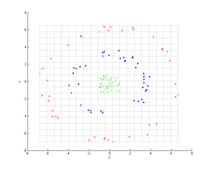
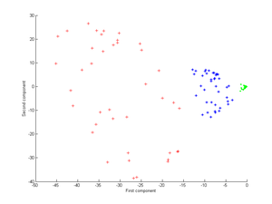
Principal component analysis (PCA) is a popular technique for analyzing large datasets containing a high number of dimensions/features per observation, increasing the interpretability of data while preserving the maximum amount of information, and enabling the visualization of multidimensional data. Formally, PCA is a statistical technique for reducing the dimensionality of a dataset. This is accomplished by linearly transforming the data into a new coordinate system where the variation in the data can be described with fewer dimensions than the initial data. Many studies use the first two principal components in order to plot the data in two dimensions and to visually identify clusters of closely related data points. Principal component analysis has applications in many fields such as population genetics, microbiome studies, and atmospheric science.
In physics, an operator is a function over a space of physical states onto another space of physical states. The simplest example of the utility of operators is the study of symmetry. Because of this, they are very useful tools in classical mechanics. Operators are even more important in quantum mechanics, where they form an intrinsic part of the formulation of the theory.

Nonlinear dimensionality reduction, also known as manifold learning, refers to various related techniques that aim to project high-dimensional data onto lower-dimensional latent manifolds, with the goal of either visualizing the data in the low-dimensional space, or learning the mapping itself. The techniques described below can be understood as generalizations of linear decomposition methods used for dimensionality reduction, such as singular value decomposition and principal component analysis.

An eigenface is the name given to a set of eigenvectors when used in the computer vision problem of human face recognition. The approach of using eigenfaces for recognition was developed by Sirovich and Kirby and used by Matthew Turk and Alex Pentland in face classification. The eigenvectors are derived from the covariance matrix of the probability distribution over the high-dimensional vector space of face images. The eigenfaces themselves form a basis set of all images used to construct the covariance matrix. This produces dimension reduction by allowing the smaller set of basis images to represent the original training images. Classification can be achieved by comparing how faces are represented by the basis set.
In the theory of stochastic processes, the Karhunen–Loève theorem, also known as the Kosambi–Karhunen–Loève theorem is a representation of a stochastic process as an infinite linear combination of orthogonal functions, analogous to a Fourier series representation of a function on a bounded interval. The transformation is also known as Hotelling transform and eigenvector transform, and is closely related to principal component analysis (PCA) technique widely used in image processing and in data analysis in many fields.

In geometry, Euler's rotation theorem states that, in three-dimensional space, any displacement of a rigid body such that a point on the rigid body remains fixed, is equivalent to a single rotation about some axis that runs through the fixed point. It also means that the composition of two rotations is also a rotation. Therefore the set of rotations has a group structure, known as a rotation group.
In mathematics, the discrete Laplace operator is an analog of the continuous Laplace operator, defined so that it has meaning on a graph or a discrete grid. For the case of a finite-dimensional graph, the discrete Laplace operator is more commonly called the Laplacian matrix.
In linear algebra, an eigenvector or characteristic vector of a linear transformation is a nonzero vector that changes at most by a scalar factor when that linear transformation is applied to it. The corresponding eigenvalue, often denoted by , is the factor by which the eigenvector is scaled.

In machine learning, kernel machines are a class of algorithms for pattern analysis, whose best known member is the support-vector machine (SVM). The general task of pattern analysis is to find and study general types of relations in datasets. For many algorithms that solve these tasks, the data in raw representation have to be explicitly transformed into feature vector representations via a user-specified feature map: in contrast, kernel methods require only a user-specified kernel, i.e., a similarity function over all pairs of data points computed using Inner products. The feature map in kernel machines is infinite dimensional but only requires a finite dimensional matrix from user-input according to the Representer theorem. Kernel machines are slow to compute for datasets larger than a couple of thousand examples without parallel processing.
The point distribution model is a model for representing the mean geometry of a shape and some statistical modes of geometric variation inferred from a training set of shapes.
In statistics, principal component regression (PCR) is a regression analysis technique that is based on principal component analysis (PCA). More specifically, PCR is used for estimating the unknown regression coefficients in a standard linear regression model.
Spike-triggered covariance (STC) analysis is a tool for characterizing a neuron's response properties using the covariance of stimuli that elicit spikes from a neuron. STC is related to the spike-triggered average (STA), and provides a complementary tool for estimating linear filters in a linear-nonlinear-Poisson (LNP) cascade model. Unlike STA, the STC can be used to identify a multi-dimensional feature space in which a neuron computes its response.
In statistics, kernel Fisher discriminant analysis (KFD), also known as generalized discriminant analysis and kernel discriminant analysis, is a kernelized version of linear discriminant analysis (LDA). It is named after Ronald Fisher.

Diffusion maps is a dimensionality reduction or feature extraction algorithm introduced by Coifman and Lafon which computes a family of embeddings of a data set into Euclidean space whose coordinates can be computed from the eigenvectors and eigenvalues of a diffusion operator on the data. The Euclidean distance between points in the embedded space is equal to the "diffusion distance" between probability distributions centered at those points. Different from linear dimensionality reduction methods such as principal component analysis (PCA), diffusion maps are part of the family of nonlinear dimensionality reduction methods which focus on discovering the underlying manifold that the data has been sampled from. By integrating local similarities at different scales, diffusion maps give a global description of the data-set. Compared with other methods, the diffusion map algorithm is robust to noise perturbation and computationally inexpensive.
Within bayesian statistics for machine learning, kernel methods arise from the assumption of an inner product space or similarity structure on inputs. For some such methods, such as support vector machines (SVMs), the original formulation and its regularization were not Bayesian in nature. It is helpful to understand them from a Bayesian perspective. Because the kernels are not necessarily positive semidefinite, the underlying structure may not be inner product spaces, but instead more general reproducing kernel Hilbert spaces. In Bayesian probability kernel methods are a key component of Gaussian processes, where the kernel function is known as the covariance function. Kernel methods have traditionally been used in supervised learning problems where the input space is usually a space of vectors while the output space is a space of scalars. More recently these methods have been extended to problems that deal with multiple outputs such as in multi-task learning.
Functional principal component analysis (FPCA) is a statistical method for investigating the dominant modes of variation of functional data. Using this method, a random function is represented in the eigenbasis, which is an orthonormal basis of the Hilbert space L2 that consists of the eigenfunctions of the autocovariance operator. FPCA represents functional data in the most parsimonious way, in the sense that when using a fixed number of basis functions, the eigenfunction basis explains more variation than any other basis expansion. FPCA can be applied for representing random functions, or in functional regression and classification.
Kernel methods are a well-established tool to analyze the relationship between input data and the corresponding output of a function. Kernels encapsulate the properties of functions in a computationally efficient way and allow algorithms to easily swap functions of varying complexity.
In statistics, modes of variation are a continuously indexed set of vectors or functions that are centered at a mean and are used to depict the variation in a population or sample. Typically, variation patterns in the data can be decomposed in descending order of eigenvalues with the directions represented by the corresponding eigenvectors or eigenfunctions. Modes of variation provide a visualization of this decomposition and an efficient description of variation around the mean. Both in principal component analysis (PCA) and in functional principal component analysis (FPCA), modes of variation play an important role in visualizing and describing the variation in the data contributed by each eigencomponent. In real-world applications, the eigencomponents and associated modes of variation aid to interpret complex data, especially in exploratory data analysis (EDA).