In fluid dynamics, turbulence or turbulent flow is fluid motion characterized by chaotic changes in pressure and flow velocity. It is in contrast to a laminar flow, which occurs when a fluid flows in parallel layers, with no disruption between those layers.

In physics and fluid mechanics, a boundary layer is the thin layer of fluid in the immediate vicinity of a bounding surface formed by the fluid flowing along the surface. The fluid's interaction with the wall induces a no-slip boundary condition. The flow velocity then monotonically increases above the surface until it returns to the bulk flow velocity. The thin layer consisting of fluid whose velocity has not yet returned to the bulk flow velocity is called the velocity boundary layer.
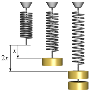
In physics, Hooke's law is an empirical law which states that the force needed to extend or compress a spring by some distance scales linearly with respect to that distance—that is, Fs = kx, where k is a constant factor characteristic of the spring, and x is small compared to the total possible deformation of the spring. The law is named after 17th-century British physicist Robert Hooke. He first stated the law in 1676 as a Latin anagram. He published the solution of his anagram in 1678 as: ut tensio, sic vis. Hooke states in the 1678 work that he was aware of the law since 1660.
A Newtonian fluid is a fluid in which the viscous stresses arising from its flow are at every point linearly correlated to the local strain rate — the rate of change of its deformation over time. Stresses are proportional to the rate of change of the fluid's velocity vector.
Quantum turbulence is the name given to the turbulent flow – the chaotic motion of a fluid at high flow rates – of quantum fluids, such as superfluids. The idea that a form of turbulence might be possible in a superfluid via the quantized vortex lines was first suggested by Richard Feynman. The dynamics of quantum fluids are governed by quantum mechanics, rather than classical physics which govern classical (ordinary) fluids. Some examples of quantum fluids include superfluid helium, Bose–Einstein condensates (BECs), polariton condensates, and nuclear pasta theorized to exist inside neutron stars. Quantum fluids exist at temperatures below the critical temperature at which Bose-Einstein condensation takes place.

Large eddy simulation (LES) is a mathematical model for turbulence used in computational fluid dynamics. It was initially proposed in 1963 by Joseph Smagorinsky to simulate atmospheric air currents, and first explored by Deardorff (1970). LES is currently applied in a wide variety of engineering applications, including combustion, acoustics, and simulations of the atmospheric boundary layer.
In fluid dynamics, the Reynolds stress is the component of the total stress tensor in a fluid obtained from the averaging operation over the Navier–Stokes equations to account for turbulent fluctuations in fluid momentum.
In fluid dynamics, turbulence modeling is the construction and use of a mathematical model to predict the effects of turbulence. Turbulent flows are commonplace in most real-life scenarios. In spite of decades of research, there is no analytical theory to predict the evolution of these turbulent flows. The equations governing turbulent flows can only be solved directly for simple cases of flow. For most real-life turbulent flows, CFD simulations use turbulent models to predict the evolution of turbulence. These turbulence models are simplified constitutive equations that predict the statistical evolution of turbulent flows.
A direct numerical simulation (DNS) is a simulation in computational fluid dynamics (CFD) in which the Navier–Stokes equations are numerically solved without any turbulence model. This means that the whole range of spatial and temporal scales of the turbulence must be resolved. All the spatial scales of the turbulence must be resolved in the computational mesh, from the smallest dissipative scales, up to the integral scale , associated with the motions containing most of the kinetic energy. The Kolmogorov scale, , is given by
In physics and fluid mechanics, a Blasius boundary layer describes the steady two-dimensional laminar boundary layer that forms on a semi-infinite plate which is held parallel to a constant unidirectional flow. Falkner and Skan later generalized Blasius' solution to wedge flow, i.e. flows in which the plate is not parallel to the flow.
In fluid dynamics, turbulence kinetic energy (TKE) is the mean kinetic energy per unit mass associated with eddies in turbulent flow. Physically, the turbulence kinetic energy is characterized by measured root-mean-square (RMS) velocity fluctuations. In the Reynolds-averaged Navier Stokes equations, the turbulence kinetic energy can be calculated based on the closure method, i.e. a turbulence model.

Preferential concentration is the tendency of dense particles in a turbulent fluid to cluster in regions of high strain due to their inertia. The extent by which particles cluster is determined by the Stokes number, defined as , where and are the timescales for the particle and fluid respectively; note that and are the mass densities of the fluid and the particle, respectively, is the kinematic viscosity of the fluid, and is the kinetic energy dissipation rate of the turbulence. Maximum preferential concentration occurs at . Particles with follow fluid streamlines and particles with do not respond significantly to the fluid within the times the fluid motions are coherent.
The Herschel–Bulkley fluid is a generalized model of a non-Newtonian fluid, in which the strain experienced by the fluid is related to the stress in a complicated, non-linear way. Three parameters characterize this relationship: the consistency k, the flow index n, and the yield shear stress . The consistency is a simple constant of proportionality, while the flow index measures the degree to which the fluid is shear-thinning or shear-thickening. Ordinary paint is one example of a shear-thinning fluid, while oobleck provides one realization of a shear-thickening fluid. Finally, the yield stress quantifies the amount of stress that the fluid may experience before it yields and begins to flow.

In fluid dynamics, vortex stretching is the lengthening of vortices in three-dimensional fluid flow, associated with a corresponding increase of the component of vorticity in the stretching direction—due to the conservation of angular momentum.
In fluid dynamics, the Taylor microscale, which is sometimes called the turbulence length scale, is a length scale used to characterize a turbulent fluid flow. This microscale is named after Geoffrey Ingram Taylor. The Taylor microscale is the intermediate length scale at which fluid viscosity significantly affects the dynamics of turbulent eddies in the flow. This length scale is traditionally applied to turbulent flow which can be characterized by a Kolmogorov spectrum of velocity fluctuations. In such a flow, length scales which are larger than the Taylor microscale are not strongly affected by viscosity. These larger length scales in the flow are generally referred to as the inertial range. Below the Taylor microscale the turbulent motions are subject to strong viscous forces and kinetic energy is dissipated into heat. These shorter length scale motions are generally termed the dissipation range.
In fluid and molecular dynamics, the Batchelor scale, determined by George Batchelor (1959), describes the size of a droplet of fluid that will diffuse in the same time it takes the energy in an eddy of size η to dissipate. The Batchelor scale can be determined by:
Magnetohydrodynamic turbulence concerns the chaotic regimes of magnetofluid flow at high Reynolds number. Magnetohydrodynamics (MHD) deals with what is a quasi-neutral fluid with very high conductivity. The fluid approximation implies that the focus is on macro length-and-time scales which are much larger than the collision length and collision time respectively.
K-epsilon (k-ε) turbulence model is one of the most common models used in computational fluid dynamics (CFD) to simulate mean flow characteristics for turbulent flow conditions. It is a two equation model that gives a general description of turbulence by means of two transport equations. The original impetus for the K-epsilon model was to improve the mixing-length model, as well as to find an alternative to algebraically prescribing turbulent length scales in moderate to high complexity flows.
Reynolds stress equation model (RSM), also referred to as second moment closures are the most complete classical turbulence model. In these models, the eddy-viscosity hypothesis is avoided and the individual components of the Reynolds stress tensor are directly computed. These models use the exact Reynolds stress transport equation for their formulation. They account for the directional effects of the Reynolds stresses and the complex interactions in turbulent flows. Reynolds stress models offer significantly better accuracy than eddy-viscosity based turbulence models, while being computationally cheaper than Direct Numerical Simulations (DNS) and Large Eddy Simulations.

In continuum mechanics, an energy cascade involves the transfer of energy from large scales of motion to the small scales or a transfer of energy from the small scales to the large scales. This transfer of energy between different scales requires that the dynamics of the system is nonlinear. Strictly speaking, a cascade requires the energy transfer to be local in scale, evoking a cascading waterfall from pool to pool without long-range transfers across the scale domain.


