
A centripetal force is a force that makes a body follow a curved path. The direction of the centripetal force is always orthogonal to the motion of the body and towards the fixed point of the instantaneous center of curvature of the path. Isaac Newton described it as "a force by which bodies are drawn or impelled, or in any way tend, towards a point as to a centre". In the theory of Newtonian mechanics, gravity provides the centripetal force causing astronomical orbits.

In physics and mathematics, in the area of dynamical systems, a double pendulum also known as a chaos pendulum is a pendulum with another pendulum attached to its end, forming a simple physical system that exhibits rich dynamic behavior with a strong sensitivity to initial conditions. The motion of a double pendulum is governed by a set of coupled ordinary differential equations and is chaotic.
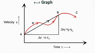
In physics, equations of motion are equations that describe the behavior of a physical system in terms of its motion as a function of time. More specifically, the equations of motion describe the behavior of a physical system as a set of mathematical functions in terms of dynamic variables. These variables are usually spatial coordinates and time, but may include momentum components. The most general choice are generalized coordinates which can be any convenient variables characteristic of the physical system. The functions are defined in a Euclidean space in classical mechanics, but are replaced by curved spaces in relativity. If the dynamics of a system is known, the equations are the solutions for the differential equations describing the motion of the dynamics.

In mathematics, the Lyapunov exponent or Lyapunov characteristic exponent of a dynamical system is a quantity that characterizes the rate of separation of infinitesimally close trajectories. Quantitatively, two trajectories in phase space with initial separation vector diverge at a rate given by
In the theory of ordinary differential equations (ODEs), Lyapunov functions, named after Aleksandr Lyapunov, are scalar functions that may be used to prove the stability of an equilibrium of an ODE. Lyapunov functions are important to stability theory of dynamical systems and control theory. A similar concept appears in the theory of general state space Markov chains, usually under the name Foster–Lyapunov functions.
Various types of stability may be discussed for the solutions of differential equations or difference equations describing dynamical systems. The most important type is that concerning the stability of solutions near to a point of equilibrium. This may be discussed by the theory of Aleksandr Lyapunov. In simple terms, if the solutions that start out near an equilibrium point stay near forever, then is Lyapunov stable. More strongly, if is Lyapunov stable and all solutions that start out near converge to , then is said to be asymptotically stable. The notion of exponential stability guarantees a minimal rate of decay, i.e., an estimate of how quickly the solutions converge. The idea of Lyapunov stability can be extended to infinite-dimensional manifolds, where it is known as structural stability, which concerns the behavior of different but "nearby" solutions to differential equations. Input-to-state stability (ISS) applies Lyapunov notions to systems with inputs.
In control systems, sliding mode control (SMC), originated by Vadim I. Utkin, is a nonlinear control method that alters the dynamics of a nonlinear system by applying a discontinuous control signal that forces the system to "slide" along a cross-section of the system's normal behaviour. The state-feedback control law is not a continuous function of time. Instead, it can switch from one continuous structure to another based on the current position in the state space. Hence, sliding mode control is a variable structure control method. The multiple control structures are designed so that trajectories always move toward an adjacent region with a different control structure, and so the ultimate trajectory will not exist entirely within one control structure. Instead, it will slide along the boundaries of the control structures. The motion of the system as it slides along these boundaries is called a sliding mode and the geometrical locus consisting of the boundaries is called the sliding (hyper)surface. In the context of modern control theory, any variable structure system, like a system under SMC, may be viewed as a special case of a hybrid dynamical system as the system both flows through a continuous state space but also moves through different discrete control modes.
In analytical mechanics, generalized coordinates are a set of parameters used to represent the state of a system in a configuration space. These parameters must uniquely define the configuration of the system relative to a reference state. The generalized velocities are the time derivatives of the generalized coordinates of the system. The adjective "generalized" distinguishes these parameters from the traditional use of the term "coordinate" to refer to Cartesian coordinates.
In control engineering and system identification, a state-space representation is a mathematical model of a physical system specified as a set of input, output and variables related by first-order differential equations or difference equations. Such variables, called state variables, evolve over time in a way that depends on the values they have at any given instant and on the externally imposed values of input variables. Output variables’ values depend on the values of the state variables and may also depend on the values of the input variables.
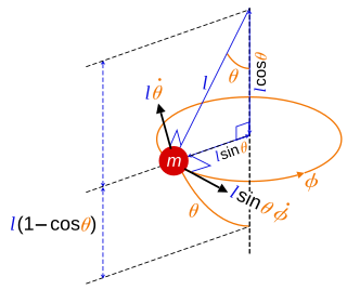
In physics, a spherical pendulum is a higher dimensional analogue of the pendulum. It consists of a mass m moving without friction on the surface of a sphere. The only forces acting on the mass are the reaction from the sphere and gravity.
In physics, the Hamilton–Jacobi equation, named after William Rowan Hamilton and Carl Gustav Jacob Jacobi, is an alternative formulation of classical mechanics, equivalent to other formulations such as Newton's laws of motion, Lagrangian mechanics and Hamiltonian mechanics.

In physics, Hamilton's principle is William Rowan Hamilton's formulation of the principle of stationary action. It states that the dynamics of a physical system are determined by a variational problem for a functional based on a single function, the Lagrangian, which may contain all physical information concerning the system and the forces acting on it. The variational problem is equivalent to and allows for the derivation of the differential equations of motion of the physical system. Although formulated originally for classical mechanics, Hamilton's principle also applies to classical fields such as the electromagnetic and gravitational fields, and plays an important role in quantum mechanics, quantum field theory and criticality theories.

In mathematics, stability theory addresses the stability of solutions of differential equations and of trajectories of dynamical systems under small perturbations of initial conditions. The heat equation, for example, is a stable partial differential equation because small perturbations of initial data lead to small variations in temperature at a later time as a result of the maximum principle. In partial differential equations one may measure the distances between functions using Lp norms or the sup norm, while in differential geometry one may measure the distance between spaces using the Gromov–Hausdorff distance.

A pendulum is a body suspended from a fixed support so that it swings freely back and forth under the influence of gravity. When a pendulum is displaced sideways from its resting, equilibrium position, it is subject to a restoring force due to gravity that will accelerate it back towards the equilibrium position. When released, the restoring force acting on the pendulum's mass causes it to oscillate about the equilibrium position, swinging it back and forth. The mathematics of pendulums are in general quite complicated. Simplifying assumptions can be made, which in the case of a simple pendulum allow the equations of motion to be solved analytically for small-angle oscillations.
In control theory, a control-Lyapunov function (CLF) is an extension of the idea of Lyapunov function to systems with control inputs. The ordinary Lyapunov function is used to test whether a dynamical system is (Lyapunov) stable or asymptotically stable. Lyapunov stability means that if the system starts in a state in some domain D, then the state will remain in D for all time. For asymptotic stability, the state is also required to converge to . A control-Lyapunov function is used to test whether a system is asymptotically stabilizable, that is whether for any state x there exists a control such that the system can be brought to the zero state asymptotically by applying the control u.
In control theory, backstepping is a technique developed circa 1990 by Myroslav Sparavalo, Petar V. Kokotovic and others for designing stabilizing controls for a special class of nonlinear dynamical systems. These systems are built from subsystems that radiate out from an irreducible subsystem that can be stabilized using some other method. Because of this recursive structure, the designer can start the design process at the known-stable system and "back out" new controllers that progressively stabilize each outer subsystem. The process terminates when the final external control is reached. Hence, this process is known as backstepping.
In nonlinear control and stability theory, the circle criterion is a stability criterion for nonlinear time-varying systems. It can be viewed as a generalization of the Nyquist stability criterion for linear time-invariant (LTI) systems.
In control theory, dynamical systems are in strict-feedback form when they can be expressed as

In physics, Lagrangian mechanics is a formulation of classical mechanics founded on the stationary-action principle. It was introduced by the Italian-French mathematician and astronomer Joseph-Louis Lagrange in his presentation to the Turin Academy of Science in 1760 culminating in his 1788 grand opus, Mécanique analytique.
Input-to-state stability (ISS) is a stability notion widely used to study stability of nonlinear control systems with external inputs. Roughly speaking, a control system is ISS if it is globally asymptotically stable in the absence of external inputs and if its trajectories are bounded by a function of the size of the input for all sufficiently large times. The importance of ISS is due to the fact that the concept has bridged the gap between input–output and state-space methods, widely used within the control systems community.


