Stability theory

Last updated
Stability diagram classifying Poincare maps of linear autonomous system
x
'
=
A
x
,
{\displaystyle x'=Ax,}
as stable or unstable according to their features. Stability generally increases to the left of the diagram. Some sink, source or node are equilibrium points. Stability Diagram.png
Stability diagram classifying Poincaré maps of linear autonomous system as stable or unstable according to their features. Stability generally increases to the left of the diagram. Some sink, source or node are equilibrium points.

In mathematics, stability theory addresses the stability of solutions of differential equations and of trajectories of dynamical systems under small perturbations of initial conditions. The heat equation, for example, is a stable partial differential equation because small perturbations of initial data lead to small variations in temperature at a later time as a result of the maximum principle. In partial differential equations one may measure the distances between functions using Lp norms or the sup norm, while in differential geometry one may measure the distance between spaces using the Gromov–Hausdorff distance.

Contents

In dynamical systems, an orbit is called Lyapunov stable if the forward orbit of any point is in a small enough neighborhood or it stays in a small (but perhaps, larger) neighborhood. Various criteria have been developed to prove stability or instability of an orbit. Under favorable circumstances, the question may be reduced to a well-studied problem involving eigenvalues of matrices. A more general method involves Lyapunov functions. In practice, any one of a number of different stability criteria are applied.

Overview in dynamical systems

Many parts of the qualitative theory of differential equations and dynamical systems deal with asymptotic properties of solutions and the trajectories—what happens with the system after a long period of time. The simplest kind of behavior is exhibited by equilibrium points, or fixed points, and by periodic orbits. If a particular orbit is well understood, it is natural to ask next whether a small change in the initial condition will lead to similar behavior. Stability theory addresses the following questions: Will a nearby orbit indefinitely stay close to a given orbit? Will it converge to the given orbit? In the former case, the orbit is called stable; in the latter case, it is called asymptotically stable and the given orbit is said to be attracting.

An equilibrium solution to an autonomous system of first order ordinary differential equations is called:

Stability means that the trajectories do not change too much under small perturbations. The opposite situation, where a nearby orbit is getting repelled from the given orbit, is also of interest. In general, perturbing the initial state in some directions results in the trajectory asymptotically approaching the given one and in other directions to the trajectory getting away from it. There may also be directions for which the behavior of the perturbed orbit is more complicated (neither converging nor escaping completely), and then stability theory does not give sufficient information about the dynamics.

One of the key ideas in stability theory is that the qualitative behavior of an orbit under perturbations can be analyzed using the linearization of the system near the orbit. In particular, at each equilibrium of a smooth dynamical system with an n-dimensional phase space, there is a certain n×n matrix A whose eigenvalues characterize the behavior of the nearby points (Hartman–Grobman theorem). More precisely, if all eigenvalues are negative real numbers or complex numbers with negative real parts then the point is a stable attracting fixed point, and the nearby points converge to it at an exponential rate, cf Lyapunov stability and exponential stability. If none of the eigenvalues are purely imaginary (or zero) then the attracting and repelling directions are related to the eigenspaces of the matrix A with eigenvalues whose real part is negative and, respectively, positive. Analogous statements are known for perturbations of more complicated orbits.

Stability of fixed points in 2D

Schematic visualization of 4 of the most common kinds of fixed points. Fixed Points.gif
Schematic visualization of 4 of the most common kinds of fixed points.

The paradigmatic case is the stability of the origin under the linear autonomous differential equation where and is a 2-by-2 matrix.

We would sometimes perform change-of-basis by for some invertible matrix , which gives . We say is " in the new basis". Since and , we can classify the stability of origin using and , while freely using change-of-basis.

Classification of stability types

If , then the rank of is zero or one.

If , we first find the Jordan normal form of the matrix, to obtain a basis in which is one of three possible forms:

The summary is shown in the stability diagram on the right. In each case, except the case of , the values allows unique classification of the type of flow.

For the special case of , there are two cases that cannot be distinguished by . In both cases, has only one eigenvalue, with algebraic multiplicity 2.

Area-preserving flow

When , we have , so the flow is area-preserving. In this case, the type of flow is classified by .

Stability of fixed points

The simplest kind of an orbit is a fixed point, or an equilibrium. If a mechanical system is in a stable equilibrium state then a small push will result in a localized motion, for example, small oscillations as in the case of a pendulum. In a system with damping, a stable equilibrium state is moreover asymptotically stable. On the other hand, for an unstable equilibrium, such as a ball resting on a top of a hill, certain small pushes will result in a motion with a large amplitude that may or may not converge to the original state.

There are useful tests of stability for the case of a linear system. Stability of a nonlinear system can often be inferred from the stability of its linearization.

Maps

Let f: RR be a continuously differentiable function with a fixed point a, f(a) = a. Consider the dynamical system obtained by iterating the function f:

The fixed point a is stable if the absolute value of the derivative of f at a is strictly less than 1, and unstable if it is strictly greater than 1. This is because near the point a, the function f has a linear approximation with slope f'(a):

Thus

which means that the derivative measures the rate at which the successive iterates approach the fixed point a or diverge from it. If the derivative at a is exactly 1 or −1, then more information is needed in order to decide stability.

There is an analogous criterion for a continuously differentiable map f: RnRn with a fixed point a, expressed in terms of its Jacobian matrix at a, Ja(f). If all eigenvalues of J are real or complex numbers with absolute value strictly less than 1 then a is a stable fixed point; if at least one of them has absolute value strictly greater than 1 then a is unstable. Just as for n=1, the case of the largest absolute value being 1 needs to be investigated further — the Jacobian matrix test is inconclusive. The same criterion holds more generally for diffeomorphisms of a smooth manifold.

Linear autonomous systems

The stability of fixed points of a system of constant coefficient linear differential equations of first order can be analyzed using the eigenvalues of the corresponding matrix.

An autonomous system

where x(t) ∈ Rn and A is an n×n matrix with real entries, has a constant solution

(In a different language, the origin 0 ∈ Rn is an equilibrium point of the corresponding dynamical system.) This solution is asymptotically stable as t → ∞ ("in the future") if and only if for all eigenvalues λ of A, Re(λ) < 0. Similarly, it is asymptotically stable as t → −∞ ("in the past") if and only if for all eigenvalues λ of A, Re(λ) > 0. If there exists an eigenvalue λ of A with Re(λ) > 0 then the solution is unstable for t → ∞.

Application of this result in practice, in order to decide the stability of the origin for a linear system, is facilitated by the Routh–Hurwitz stability criterion. The eigenvalues of a matrix are the roots of its characteristic polynomial. A polynomial in one variable with real coefficients is called a Hurwitz polynomial if the real parts of all roots are strictly negative. The Routh–Hurwitz theorem implies a characterization of Hurwitz polynomials by means of an algorithm that avoids computing the roots.

Non-linear autonomous systems

Asymptotic stability of fixed points of a non-linear system can often be established using the Hartman–Grobman theorem.

Suppose that v is a C1-vector field in Rn which vanishes at a point p, v(p) = 0. Then the corresponding autonomous system

has a constant solution

Let Jp(v) be the n×n Jacobian matrix of the vector field v at the point p. If all eigenvalues of J have strictly negative real part then the solution is asymptotically stable. This condition can be tested using the Routh–Hurwitz criterion.

Lyapunov function for general dynamical systems

A general way to establish Lyapunov stability or asymptotic stability of a dynamical system is by means of Lyapunov functions.

See also

Related Research Articles

In mathematics, the determinant is a scalar value that is a certain function of the entries of a square matrix. The determinant of a matrix A is commonly denoted det(A), det A, or |A|. Its value characterizes some properties of the matrix and the linear map represented, on a given basis, by the matrix. In particular, the determinant is nonzero if and only if the matrix is invertible and the corresponding linear map is an isomorphism. The determinant of a product of matrices is the product of their determinants.

<span class="mw-page-title-main">Pauli matrices</span> Matrices important in quantum mechanics and the study of spin

In mathematical physics and mathematics, the Pauli matrices are a set of three 2 × 2 complex matrices that are Hermitian, involutory and unitary. Usually indicated by the Greek letter sigma, they are occasionally denoted by tau when used in connection with isospin symmetries.

In mathematics, a symmetric matrix with real entries is positive-definite if the real number is positive for every nonzero real column vector where is the transpose of . More generally, a Hermitian matrix is positive-definite if the real number is positive for every nonzero complex column vector where denotes the conjugate transpose of

<span class="mw-page-title-main">Ellipsoid</span> Quadric surface that looks like a deformed sphere

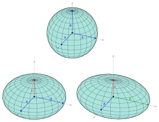
An ellipsoid is a surface that can be obtained from a sphere by deforming it by means of directional scalings, or more generally, of an affine transformation.

Ray transfer matrix analysis is a mathematical form for performing ray tracing calculations in sufficiently simple problems which can be solved considering only paraxial rays. Each optical element is described by a 2×2 ray transfer matrix which operates on a vector describing an incoming light ray to calculate the outgoing ray. Multiplication of the successive matrices thus yields a concise ray transfer matrix describing the entire optical system. The same mathematics is also used in accelerator physics to track particles through the magnet installations of a particle accelerator, see electron optics.

<span class="mw-page-title-main">Orthogonal group</span> Type of group in mathematics

In mathematics, the orthogonal group in dimension n, denoted O(n), is the group of distance-preserving transformations of a Euclidean space of dimension n that preserve a fixed point, where the group operation is given by composing transformations. The orthogonal group is sometimes called the general orthogonal group, by analogy with the general linear group. Equivalently, it is the group of n × n orthogonal matrices, where the group operation is given by matrix multiplication (an orthogonal matrix is a real matrix whose inverse equals its transpose). The orthogonal group is an algebraic group and a Lie group. It is compact.

In mechanics and geometry, the 3D rotation group, often denoted SO(3), is the group of all rotations about the origin of three-dimensional Euclidean space under the operation of composition.

In mathematics, particularly in linear algebra, a skew-symmetricmatrix is a square matrix whose transpose equals its negative. That is, it satisfies the condition

In vector calculus, the Jacobian matrix of a vector-valued function of several variables is the matrix of all its first-order partial derivatives. When this matrix is square, that is, when the function takes the same number of variables as input as the number of vector components of its output, its determinant is referred to as the Jacobian determinant. Both the matrix and the determinant are often referred to simply as the Jacobian in literature.

In mathematics, the conjugate transpose, also known as the Hermitian transpose, of an complex matrix is an matrix obtained by transposing and applying complex conjugation to each entry. There are several notations, such as or , , or .

In mathematics, a Gaussian function, often simply referred to as a Gaussian, is a function of the base form

<span class="mw-page-title-main">Jordan normal form</span> Form of a matrix indicating its eigenvalues and their algebraic multiplicities

In linear algebra, a Jordan normal form, also known as a Jordan canonical form (JCF), is an upper triangular matrix of a particular form called a Jordan matrix representing a linear operator on a finite-dimensional vector space with respect to some basis. Such a matrix has each non-zero off-diagonal entry equal to 1, immediately above the main diagonal, and with identical diagonal entries to the left and below them.

In mathematics, the determinant of an m×m skew-symmetric matrix can always be written as the square of a polynomial in the matrix entries, a polynomial with integer coefficients that only depends on m. When m is odd, the polynomial is zero. When m is even, it is a nonzero polynomial of degree m/2, and is unique up to multiplication by ±1. The convention on skew-symmetric tridiagonal matrices, given below in the examples, then determines one specific polynomial, called the Pfaffian polynomial. The value of this polynomial, when applied to the entries of a skew-symmetric matrix, is called the Pfaffian of that matrix. The term Pfaffian was introduced by Cayley, who indirectly named them after Johann Friedrich Pfaff.

In mathematical statistics, the Fisher information is a way of measuring the amount of information that an observable random variable X carries about an unknown parameter θ of a distribution that models X. Formally, it is the variance of the score, or the expected value of the observed information.

In mathematics, the matrix exponential is a matrix function on square matrices analogous to the ordinary exponential function. It is used to solve systems of linear differential equations. In the theory of Lie groups, the matrix exponential gives the exponential map between a matrix Lie algebra and the corresponding Lie group.

In linear algebra, a rotation matrix is a transformation matrix that is used to perform a rotation in Euclidean space. For example, using the convention below, the matrix

In statistics, ordinary least squares (OLS) is a type of linear least squares method for choosing the unknown parameters in a linear regression model by the principle of least squares: minimizing the sum of the squares of the differences between the observed dependent variable in the input dataset and the output of the (linear) function of the independent variable.

In linear algebra, it is often important to know which vectors have their directions unchanged by a given linear transformation. An eigenvector or characteristic vector is such a vector. Thus an eigenvector of a linear transformation is scaled by a constant factor when the linear transformation is applied to it: . The corresponding eigenvalue, characteristic value, or characteristic root is the multiplying factor .

<span class="mw-page-title-main">Hyperbolic equilibrium point</span>

In the study of dynamical systems, a hyperbolic equilibrium point or hyperbolic fixed point is a fixed point that does not have any center manifolds. Near a hyperbolic point the orbits of a two-dimensional, non-dissipative system resemble hyperbolas. This fails to hold in general. Strogatz notes that "hyperbolic is an unfortunate name—it sounds like it should mean 'saddle point'—but it has become standard." Several properties hold about a neighborhood of a hyperbolic point, notably

<span class="mw-page-title-main">Axis–angle representation</span> Parameterization of a rotation into a unit vector and angle

In mathematics, the axis–angle representation parameterizes a rotation in a three-dimensional Euclidean space by two quantities: a unit vector e indicating the direction (geometry) of an axis of rotation, and an angle of rotation θ describing the magnitude and sense of the rotation about the axis. Only two numbers, not three, are needed to define the direction of a unit vector e rooted at the origin because the magnitude of e is constrained. For example, the elevation and azimuth angles of e suffice to locate it in any particular Cartesian coordinate frame.

References

  1. Egwald Mathematics - Linear Algebra: Systems of Linear Differential Equations: Linear Stability Analysis Accessed 10 October 2019.
  2. "Node - Encyclopedia of Mathematics". encyclopediaofmath.org. Retrieved 2023-03-30.