Ikeda map

Last updated April 22, 2024

In physics and mathematics, the Ikeda map is a discrete-time dynamical system given by the complex map

The original map was proposed first by Kensuke Ikeda as a model of light going around across a nonlinear optical resonator (ring cavity containing a nonlinear ^{[ disambiguation needed ]} dielectric medium) in a more general form. It is reduced to the above simplified "normal" form by Ikeda, Daido and Akimoto ^[1]^[2] $z_{n}$ stands for the electric field inside the resonator at the n-th step of rotation in the resonator, and $A$ and $C$ are parameters which indicate laser light applied from the outside, and linear phase across the resonator, respectively. In particular the parameter $B\leq 1$ is called dissipation parameter characterizing the loss of resonator, and in the limit of $B=1$ the Ikeda map becomes a conservative map.

The original Ikeda map is often used in another modified form in order to take the saturation effect of nonlinear dielectric medium into account:

z_{n+1}=A+Bz_{n}e^{iK/(|z_{n}|^{2}+1)+C}

A 2D real example of the above form is:

x_{n+1}=1+u(x_{n}\cos t_{n}-y_{n}\sin t_{n}),\,

y_{n+1}=u(x_{n}\sin t_{n}+y_{n}\cos t_{n}),

where u is a parameter and

t_{n}=0.4-{\frac {6}{1+x_{n}^{2}+y_{n}^{2}}}.

For $u\geq 0.6$ , this system has a chaotic attractor.

Attractor

This animation shows how the attractor of the system changes as the parameter $u$ is varied from 0.0 to 1.0 in steps of 0.01. The Ikeda dynamical system is simulated for 500 steps, starting from 20000 randomly placed starting points. The last 20 points of each trajectory are plotted to depict the attractor. Note the bifurcation of attractor points as $u$ is increased.

$u = 0.3 {\displaystyle u=0.3} Ikeda0300.png$ $u=0.3$	$u = 0.5 {\displaystyle u=0.5} Ikeda0500.png$ $u=0.5$
$u = 0.7 {\displaystyle u=0.7} Ikeda0700.png$ $u=0.7$	$u = 0.9 {\displaystyle u=0.9} Ikeda0900.png$ $u=0.9$

Point trajectories

The plots below show trajectories of 200 random points for various values of $u$ . The inset plot on the left shows an estimate of the attractor while the inset on the right shows a zoomed in view of the main trajectory plot.

u = 0.1	u = 0.5	u = 0.65
u = 0.7	u = 0.8	u = 0.85
u = 0.9	u = 0.908	u = 0.92

Octave/MATLAB code for point trajectories

The Ikeda map is composed by a rotation (by a radius-dependent angle), a rescaling, and a shift. This "stretch and fold" process gives rise to the strange attractor.

The Octave/MATLAB code to generate these plots is given below:

% u = ikeda parameter% option = what to plot%  'trajectory' - plot trajectory of random starting points%  'limit' - plot the last few iterations of random starting pointsfunctionikeda(u, option)P=200;% how many starting pointsN=1000;% how many iterationsNlimit=20;% plot these many last points for 'limit' optionx=randn(1,P)*10;% the random starting pointsy=randn(1,P)*10;forn=1:P,X=compute_ikeda_trajectory(u,x(n),y(n),N);switchoptioncase'trajectory'% plot the trajectories of a bunch of pointsplot_ikeda_trajectory(X);holdon;case'limit'plot_limit(X,Nlimit);holdon;otherwisedisp('Not implemented');endendaxistight;axisequaltext(-25,-15,['u = 'num2str(u)]);text(-25,-18,['N = 'num2str(N)' iterations']);end% Plot the last n points of the curve - to see end point or limit cyclefunctionplot_limit(X, n)plot(X(end-n:end,1),X(end-n:end,2),'ko');end% Plot the whole trajectoryfunctionplot_ikeda_trajectory(X)plot(X(:,1),X(:,2),'k');% hold on; plot(X(1,1), X(1,2), 'bo', 'markerfacecolor', 'g'); hold offend% u is the ikeda parameter% x,y is the starting point% N is the number of iterationsfunction[X]=compute_ikeda_trajectory(u, x, y, N)X=zeros(N,2);X(1,:)=[xy];forn=2:Nt=0.4-6/(1+x^2+y^2);x1=1+u*(x*cos(t)-y*sin(t));y1=u*(x*sin(t)+y*cos(t));x=x1;y=y1;X(n,:)=[xy];endend

Python code for point trajectories

importmathimportmatplotlib.pyplotaspltimportnumpyasnpdefmain(u:float,points=200,iterations=1000,nlim=20,limit=False,title=True):"""    Args:        u:float            ikeda parameter        points:int            number of starting points        iterations:int            number of iterations        nlim:int            plot these many last points for 'limit' option. Will plot all points if set to zero        limit:bool            plot the last few iterations of random starting points if True. Else Plot trajectories.        title:[str, NoneType]            display the name of the plot if the value is affirmative    """x=10*np.random.randn(points,1)y=10*np.random.randn(points,1)forninrange(points):X=compute_ikeda_trajectory(u,x[n][0],y[n][0],iterations)iflimit:plot_limit(X,nlim)tx,ty=2.5,-1.8else:plot_ikeda_trajectory(X)tx,ty=-30,-26plt.title(f"Ikeda Map ({u=:.2g}, {iterations=})")iftitleelseNonereturnpltdefcompute_ikeda_trajectory(u:float,x:float,y:float,N:int):"""Calculate a full trajectory    Args:        u - is the ikeda parameter        x, y - coordinates of the starting point        N - the number of iterations    Returns:        An array.    """X=np.zeros((N,2))forninrange(N):X[n]=np.array((x,y))t=0.4-6/(1+x**2+y**2)x1=1+u*(x*math.cos(t)-y*math.sin(t))y1=u*(x*math.sin(t)+y*math.cos(t))x=x1y=y1returnXdefplot_limit(X,n:int)->None:"""    Plot the last n points of the curve - to see end point or limit cycle    Args:        X: np.array            trajectory of an associated starting-point        n: int            number of "last" points to plot    """plt.plot(X[-n:,0],X[-n:,1],'ko')defplot_ikeda_trajectory(X)->None:"""    Plot the whole trajectory    Args:        X: np.array            trajectory of an associated starting-point    """plt.plot(X[:,0],X[:,1],"k")if__name__=="__main__":main(0.9,limit=True,nlim=0).show()

Related Research Articles

<span class="mw-page-title-main">Ellipse</span> Plane curve: conic section

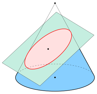
In mathematics, an ellipse is a plane curve surrounding two focal points, such that for all points on the curve, the sum of the two distances to the focal points is a constant. It generalizes a circle, which is the special type of ellipse in which the two focal points are the same. The elongation of an ellipse is measured by its eccentricity $, a number ranging from to .$

In probability theory, a probability density function (PDF), density function, or density of an absolutely continuous random variable, is a function whose value at any given sample in the sample space can be interpreted as providing a relative likelihood that the value of the random variable would be equal to that sample. Probability density is the probability per unit length, in other words, while the absolute likelihood for a continuous random variable to take on any particular value is 0, the value of the PDF at two different samples can be used to infer, in any particular draw of the random variable, how much more likely it is that the random variable would be close to one sample compared to the other sample.

In mathematics, the Lambert $W$ function, also called the omega function or product logarithm, is a multivalued function, namely the branches of the converse relation of the function $f (w) = we w$ , where $w$ is any complex number and $e w$ is the exponential function. The function is named after Johann Lambert, who considered a related problem in 1758. Building on Lambert's work, Leonhard Euler described the $W$ function per se in 1783.

In calculus, and more generally in mathematical analysis, integration by parts or partial integration is a process that finds the integral of a product of functions in terms of the integral of the product of their derivative and antiderivative. It is frequently used to transform the antiderivative of a product of functions into an antiderivative for which a solution can be more easily found. The rule can be thought of as an integral version of the product rule of differentiation; it is indeed derived using the product rule.

In mathematics, a Gaussian function, often simply referred to as a Gaussian, is a function of the base form

In mathematics, the beta function, also called the Euler integral of the first kind, is a special function that is closely related to the gamma function and to binomial coefficients. It is defined by the integral

A nonholonomic system in physics and mathematics is a physical system whose state depends on the path taken in order to achieve it. Such a system is described by a set of parameters subject to differential constraints and non-linear constraints, such that when the system evolves along a path in its parameter space but finally returns to the original set of parameter values at the start of the path, the system itself may not have returned to its original state. Nonholonomic mechanics is autonomous division of Newtonian mechanics.

In mathematics, a parametric equation defines a group of quantities as functions of one or more independent variables called parameters. Parametric equations are commonly used to express the coordinates of the points that make up a geometric object such as a curve or surface, called a parametric curve and parametric surface, respectively. In such cases, the equations are collectively called a parametric representation, or parametric system, or parameterization of the object.

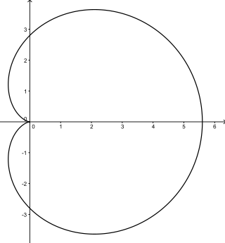
<span class="mw-page-title-main">Cardioid</span> Type of plane curve

In geometry, a cardioid is a plane curve traced by a point on the perimeter of a circle that is rolling around a fixed circle of the same radius. It can also be defined as an epicycloid having a single cusp. It is also a type of sinusoidal spiral, and an inverse curve of the parabola with the focus as the center of inversion. A cardioid can also be defined as the set of points of reflections of a fixed point on a circle through all tangents to the circle.

In the mathematical field of complex analysis, contour integration is a method of evaluating certain integrals along paths in the complex plane.

In mathematics, the Lévy C curve is a self-similar fractal curve that was first described and whose differentiability properties were analysed by Ernesto Cesàro in 1906 and Georg Faber in 1910, but now bears the name of French mathematician Paul Lévy, who was the first to describe its self-similarity properties as well as to provide a geometrical construction showing it as a representative curve in the same class as the Koch curve. It is a special case of a period-doubling curve, a de Rham curve.

Random sample consensus (RANSAC) is an iterative method to estimate parameters of a mathematical model from a set of observed data that contains outliers, when outliers are to be accorded no influence on the values of the estimates. Therefore, it also can be interpreted as an outlier detection method. It is a non-deterministic algorithm in the sense that it produces a reasonable result only with a certain probability, with this probability increasing as more iterations are allowed. The algorithm was first published by Fischler and Bolles at SRI International in 1981. They used RANSAC to solve the Location Determination Problem (LDP), where the goal is to determine the points in the space that project onto an image into a set of landmarks with known locations.

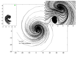
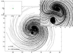
In probability theory, a distribution is said to be stable if a linear combination of two independent random variables with this distribution has the same distribution, up to location and scale parameters. A random variable is said to be stable if its distribution is stable. The stable distribution family is also sometimes referred to as the Lévy alpha-stable distribution, after Paul Lévy, the first mathematician to have studied it.

In calculus, the Leibniz integral rule for differentiation under the integral sign states that for an integral of the form

In Itô calculus, the Euler–Maruyama method is a method for the approximate numerical solution of a stochastic differential equation (SDE). It is an extension of the Euler method for ordinary differential equations to stochastic differential equations. It is named after Leonhard Euler and Gisiro Maruyama. Unfortunately, the same generalization cannot be done for any arbitrary deterministic method.

In mathematics, the Milstein method is a technique for the approximate numerical solution of a stochastic differential equation. It is named after Grigori N. Milstein who first published it in 1974.

The Marsaglia polar method is a pseudo-random number sampling method for generating a pair of independent standard normal random variables.

In mathematics, a unit circle is a circle of unit radius—that is, a radius of 1. Frequently, especially in trigonometry, the unit circle is the circle of radius 1 centered at the origin in the Cartesian coordinate system in the Euclidean plane. In topology, it is often denoted as $S 1$ because it is a one-dimensional unit $n$ -sphere.

The Lorenz 96 model is a dynamical system formulated by Edward Lorenz in 1996. It is defined as follows. For $:$

The GEKKO Python package solves large-scale mixed-integer and differential algebraic equations with nonlinear programming solvers. Modes of operation include machine learning, data reconciliation, real-time optimization, dynamic simulation, and nonlinear model predictive control. In addition, the package solves Linear programming (LP), Quadratic programming (QP), Quadratically constrained quadratic program (QCQP), Nonlinear programming (NLP), Mixed integer programming (MIP), and Mixed integer linear programming (MILP). GEKKO is available in Python and installed with pip from PyPI of the Python Software Foundation.

References

↑ Ikeda, Kensuke (1979). "Multiple-valued stationary state and its instability of the transmitted light by a ring cavity system". Optics Communications. 30 (2). Elsevier BV: 257–261. Bibcode:1979OptCo..30..257I. CiteSeerX 10.1.1.158.7964 . doi:10.1016/0030-4018(79)90090-7. ISSN 0030-4018.
↑ Ikeda, K.; Daido, H.; Akimoto, O. (1980-09-01). "Optical Turbulence: Chaotic Behavior of Transmitted Light from a Ring Cavity". Physical Review Letters. 45 (9). American Physical Society (APS): 709–712. Bibcode:1980PhRvL..45..709I. doi:10.1103/physrevlett.45.709. ISSN 0031-9007.

This page is based on this Wikipedia article
Text is available under the CC BY-SA 4.0 license; additional terms may apply.
Images, videos and audio are available under their respective licenses.

[1] Ikeda, Kensuke (1979). "Multiple-valued stationary state and its instability of the transmitted light by a ring cavity system". Optics Communications. 30 (2). Elsevier BV: 257–261. Bibcode:1979OptCo..30..257I. CiteSeerX 10.1.1.158.7964 . doi:10.1016/0030-4018(79)90090-7. ISSN 0030-4018.

[2] Ikeda, K.; Daido, H.; Akimoto, O. (1980-09-01). "Optical Turbulence: Chaotic Behavior of Transmitted Light from a Ring Cavity". Physical Review Letters. 45 (9). American Physical Society (APS): 709–712. Bibcode:1980PhRvL..45..709I. doi:10.1103/physrevlett.45.709. ISSN 0031-9007.

[1]

[2]