An LVQ system is represented by prototypes which are defined in the feature space of observed data. In winner-take-all training algorithms one determines, for each data point, the prototype which is closest to the input according to a given distance measure. The position of this so-called winner prototype is then adapted, i.e. the winner is moved closer if it correctly classifies the data point or moved away if it classifies the data point incorrectly.
An advantage of LVQ is that it creates prototypes that are easy to interpret for experts in the respective application domain.[2] LVQ systems can be applied to multi-class classification problems in a natural way.
A key issue in LVQ is the choice of an appropriate measure of distance or similarity for training and classification. Recently, techniques have been developed which adapt a parameterized distance measure in the course of training the system, see e.g. (Schneider, Biehl, and Hammer, 2009)[3] and references therein.
LVQ can be a source of great help in classifying text documents.[citation needed]
Let the data be denoted by , and their corresponding labels by .
The complete dataset is .
The set of code vectors is .
The learning rate at iteration step is denoted by .
The hyperparameters and are used by LVQ2 and LVQ3. The original paper suggests and .
LVQ1
Initialize several code vectors per label. Iterate until convergence criteria is reached.
Sample a datum , and find out the code vector , such that falls within the Voronoi cell of .
If its label is the same as that of , then , otherwise, .
LVQ2
LVQ2 is the same as LVQ3, but with this sentence removed: "If and and have the same class, then and .". If and and have the same class, then nothing happens.
LVQ3
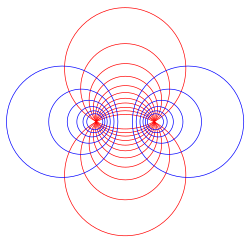
Some Apollonian circles. Every blue circle intersects every red circle at a right angle. Every red circle passes through the two points C, D, and every blue circle separates the two points.
Initialize several code vectors per label. Iterate until convergence criteria is reached.
Sample a datum , and find out two code vectors closest to it.
Let .
If , where , then
If and have the same class, and and have different classes, then and .
If and have the same class, and and have different classes, then and .
If and and have the same class, then and .
If and have different classes, and and have different classes, then the original paper simply does not explain what happens in this case, but presumably nothing happens in this case.
Otherwise, skip.
Note that condition , where , precisely means that the point falls between two Apollonian spheres.
References
↑ T. Kohonen. Self-Organizing Maps. Springer, Berlin, 1997.
↑ T. Kohonen (1995), "Learning vector quantization", in M.A. Arbib (ed.), The Handbook of Brain Theory and Neural Networks, Cambridge, MA: MIT Press, pp.537–540
lvq_pak official release (1996) by Kohonen and his team
This page is based on this Wikipedia article Text is available under the CC BY-SA 4.0 license; additional terms may apply. Images, videos and audio are available under their respective licenses.