In probability theory and statistics, the multivariate normal distribution, multivariate Gaussian distribution, or joint normal distribution is a generalization of the one-dimensional (univariate) normal distribution to higher dimensions. One definition is that a random vector is said to be k-variate normally distributed if every linear combination of its k components has a univariate normal distribution. Its importance derives mainly from the multivariate central limit theorem. The multivariate normal distribution is often used to describe, at least approximately, any set of (possibly) correlated real-valued random variables each of which clusters around a mean value.

The method of least squares is a parameters estimation method in regression analysis based on minimizing the sum of the squares of the residuals made in the results of each individual equation.
In statistics, the Gauss–Markov theorem states that the ordinary least squares (OLS) estimator has the lowest sampling variance within the class of linear unbiased estimators, if the errors in the linear regression model are uncorrelated, have equal variances and expectation value of zero. The errors do not need to be normal, nor do they need to be independent and identically distributed. The requirement that the estimator be unbiased cannot be dropped, since biased estimators exist with lower variance. See, for example, the James–Stein estimator, ridge regression, or simply any degenerate estimator.

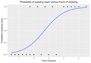
In statistics, the logistic model is a statistical model that models the log-odds of an event as a linear combination of one or more independent variables. In regression analysis, logistic regression is estimating the parameters of a logistic model. Formally, in binary logistic regression there is a single binary dependent variable, coded by an indicator variable, where the two values are labeled "0" and "1", while the independent variables can each be a binary variable or a continuous variable. The corresponding probability of the value labeled "1" can vary between 0 and 1, hence the labeling; the function that converts log-odds to probability is the logistic function, hence the name. The unit of measurement for the log-odds scale is called a logit, from logistic unit, hence the alternative names. See § Background and § Definition for formal mathematics, and § Example for a worked example.
In statistics, a studentized residual is the dimensionless ratio resulting from the division of a residual by an estimate of its standard deviation, both expressed in the same units. It is a form of a Student's t-statistic, with the estimate of error varying between points.
In statistics, a generalized linear model (GLM) is a flexible generalization of ordinary linear regression. The GLM generalizes linear regression by allowing the linear model to be related to the response variable via a link function and by allowing the magnitude of the variance of each measurement to be a function of its predicted value.

In statistical modeling, regression analysis is a set of statistical processes for estimating the relationships between a dependent variable and one or more independent variables. The most common form of regression analysis is linear regression, in which one finds the line that most closely fits the data according to a specific mathematical criterion. For example, the method of ordinary least squares computes the unique line that minimizes the sum of squared differences between the true data and that line. For specific mathematical reasons, this allows the researcher to estimate the conditional expectation of the dependent variable when the independent variables take on a given set of values. Less common forms of regression use slightly different procedures to estimate alternative location parameters or estimate the conditional expectation across a broader collection of non-linear models.

In applied statistics, total least squares is a type of errors-in-variables regression, a least squares data modeling technique in which observational errors on both dependent and independent variables are taken into account. It is a generalization of Deming regression and also of orthogonal regression, and can be applied to both linear and non-linear models.
In statistics, ordinary least squares (OLS) is a type of linear least squares method for choosing the unknown parameters in a linear regression model by the principle of least squares: minimizing the sum of the squares of the differences between the observed dependent variable in the input dataset and the output of the (linear) function of the independent variable.
Weighted least squares (WLS), also known as weighted linear regression, is a generalization of ordinary least squares and linear regression in which knowledge of the unequal variance of observations (heteroscedasticity) is incorporated into the regression. WLS is also a specialization of generalized least squares, when all the off-diagonal entries of the covariance matrix of the errors, are null.

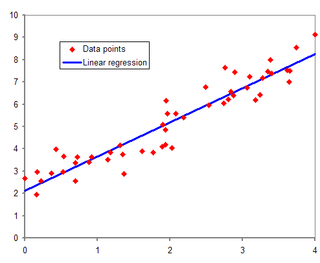
In statistics, simple linear regression (SLR) is a linear regression model with a single explanatory variable. That is, it concerns two-dimensional sample points with one independent variable and one dependent variable and finds a linear function that, as accurately as possible, predicts the dependent variable values as a function of the independent variable. The adjective simple refers to the fact that the outcome variable is related to a single predictor.
In statistics, Cook's distance or Cook's D is a commonly used estimate of the influence of a data point when performing a least-squares regression analysis. In a practical ordinary least squares analysis, Cook's distance can be used in several ways: to indicate influential data points that are particularly worth checking for validity; or to indicate regions of the design space where it would be good to be able to obtain more data points. It is named after the American statistician R. Dennis Cook, who introduced the concept in 1977.
In statistics, generalized least squares (GLS) is a method used to estimate the unknown parameters in a linear regression model when there is a certain degree of correlation between the residuals in the regression model. GLS is employed to improve statistical efficiency and reduce the risk of drawing erroneous inferences compared to conventional least squares and weighted least squares methods. It was first described by Alexander Aitken in 1935.
In statistics, Bayesian multivariate linear regression is a Bayesian approach to multivariate linear regression, i.e. linear regression where the predicted outcome is a vector of correlated random variables rather than a single scalar random variable. A more general treatment of this approach can be found in the article MMSE estimator.
The topic of heteroskedasticity-consistent (HC) standard errors arises in statistics and econometrics in the context of linear regression and time series analysis. These are also known as heteroskedasticity-robust standard errors, Eicker–Huber–White standard errors, to recognize the contributions of Friedhelm Eicker, Peter J. Huber, and Halbert White.
In statistics, the projection matrix, sometimes also called the influence matrix or hat matrix, maps the vector of response values to the vector of fitted values. It describes the influence each response value has on each fitted value. The diagonal elements of the projection matrix are the leverages, which describe the influence each response value has on the fitted value for that same observation.
In statistics, principal component regression (PCR) is a regression analysis technique that is based on principal component analysis (PCA). More specifically, PCR is used for estimating the unknown regression coefficients in a standard linear regression model.
The purpose of this page is to provide supplementary materials for the ordinary least squares article, reducing the load of the main article with mathematics and improving its accessibility, while at the same time retaining the completeness of exposition.
Linear least squares (LLS) is the least squares approximation of linear functions to data. It is a set of formulations for solving statistical problems involved in linear regression, including variants for ordinary (unweighted), weighted, and generalized (correlated) residuals. Numerical methods for linear least squares include inverting the matrix of the normal equations and orthogonal decomposition methods.

The hyperbolastic functions, also known as hyperbolastic growth models, are mathematical functions that are used in medical statistical modeling. These models were originally developed to capture the growth dynamics of multicellular tumor spheres, and were introduced in 2005 by Mohammad Tabatabai, David Williams, and Zoran Bursac. The precision of hyperbolastic functions in modeling real world problems is somewhat due to their flexibility in their point of inflection. These functions can be used in a wide variety of modeling problems such as tumor growth, stem cell proliferation, pharma kinetics, cancer growth, sigmoid activation function in neural networks, and epidemiological disease progression or regression.


