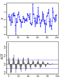
Autocorrelation, sometimes known as serial correlation in the discrete time case, is the correlation of a signal with a delayed copy of itself as a function of delay. Informally, it is the similarity between observations as a function of the time lag between them. The analysis of autocorrelation is a mathematical tool for finding repeating patterns, such as the presence of a periodic signal obscured by noise, or identifying the missing fundamental frequency in a signal implied by its harmonic frequencies. It is often used in signal processing for analyzing functions or series of values, such as time domain signals.

In statistics, correlation or dependence is any statistical relationship, whether causal or not, between two random variables or bivariate data. In the broadest sense correlation is any statistical association, though it actually refers to the degree to which a pair of variables are linearly related. Familiar examples of dependent phenomena include the correlation between the height of parents and their offspring, and the correlation between the price of a good and the quantity the consumers are willing to purchase, as it is depicted in the so-called demand curve.

In statistics, the Pearson correlation coefficient ― also known as Pearson's r, the Pearson product-moment correlation coefficient (PPMCC), the bivariate correlation, or colloquially simply as the correlation coefficient ― is a measure of linear correlation between two sets of data. It is the ratio between the covariance of two variables and the product of their standard deviations; thus it is essentially a normalised measurement of the covariance, such that the result always has a value between −1 and 1. As with covariance itself, the measure can only reflect a linear correlation of variables, and ignores many other types of relationship or correlation. As a simple example, one would expect the age and height of a sample of teenagers from a high school to have a Pearson correlation coefficient significantly greater than 0, but less than 1.
In physics, two wave sources are coherent if their frequency and waveform are identical. Coherence is an ideal property of waves that enables stationary interference. It contains several distinct concepts, which are limiting cases that never quite occur in reality but allow an understanding of the physics of waves, and has become a very important concept in quantum physics. More generally, coherence describes all properties of the correlation between physical quantities of a single wave, or between several waves or wave packets.

In astronomy, a correlation function describes the distribution of galaxies in the universe. By default, "correlation function" refers to the two-point autocorrelation function. The two-point autocorrelation function is a function of one variable (distance); it describes the excess probability of finding two galaxies separated by this distance. It can be thought of as a lumpiness factor - the higher the value for some distance scale, the more lumpy the universe is at that distance scale.

In signal processing, cross-correlation is a measure of similarity of two series as a function of the displacement of one relative to the other. This is also known as a sliding dot product or sliding inner-product. It is commonly used for searching a long signal for a shorter, known feature. It has applications in pattern recognition, single particle analysis, electron tomography, averaging, cryptanalysis, and neurophysiology. The cross-correlation is similar in nature to the convolution of two functions. In an autocorrelation, which is the cross-correlation of a signal with itself, there will always be a peak at a lag of zero, and its size will be the signal energy.
In probability theory and statistics, given a stochastic process, the autocovariance is a function that gives the covariance of the process with itself at pairs of time points. Autocovariance is closely related to the autocorrelation of the process in question.
In statistics, econometrics and signal processing, an autoregressive (AR) model is a representation of a type of random process; as such, it is used to describe certain time-varying processes in nature, economics, etc. The autoregressive model specifies that the output variable depends linearly on its own previous values and on a stochastic term ; thus the model is in the form of a stochastic difference equation. Together with the moving-average (MA) model, it is a special case and key component of the more general autoregressive–moving-average (ARMA) and autoregressive integrated moving average (ARIMA) models of time series, which have a more complicated stochastic structure; it is also a special case of the vector autoregressive model (VAR), which consists of a system of more than one interlocking stochastic difference equation in more than one evolving random variable.
A maximum length sequence (MLS) is a type of pseudorandom binary sequence.
A long-tailed or heavy-tailed probability distribution is one that assigns relatively high probabilities to regions far from the mean or median. A more formal mathematical definition is given below. In the context of teletraffic engineering a number of quantities of interest have been shown to have a long-tailed distribution. For example, if we consider the sizes of files transferred from a web-server, then, to a good degree of accuracy, the distribution is heavy-tailed, that is, there are a large number of small files transferred but, crucially, the number of very large files transferred remains a major component of the volume downloaded.
Fluorescence correlation spectroscopy (FCS) is a statistical analysis, via time correlation, of stationary fluctuations of the fluorescence intensity. Its theoretical underpinning originated from L. Onsager's regression hypothesis. The analysis provides kinetic parameters of the physical processes underlying the fluctuations. One of the interesting applications of this is an analysis of the concentration fluctuations of fluorescent particles (molecules) in solution. In this application, the fluorescence emitted from a very tiny space in solution containing a small number of fluorescent particles (molecules) is observed. The fluorescence intensity is fluctuating due to Brownian motion of the particles. In other words, the number of the particles in the sub-space defined by the optical system is randomly changing around the average number. The analysis gives the average number of fluorescent particles and average diffusion time, when the particle is passing through the space. Eventually, both the concentration and size of the particle (molecule) are determined. Both parameters are important in biochemical research, biophysics, and chemistry.
In statistics, the Durbin–Watson statistic is a test statistic used to detect the presence of autocorrelation at lag 1 in the residuals from a regression analysis. It is named after James Durbin and Geoffrey Watson. The small sample distribution of this ratio was derived by John von Neumann. Durbin and Watson applied this statistic to the residuals from least squares regressions, and developed bounds tests for the null hypothesis that the errors are serially uncorrelated against the alternative that they follow a first order autoregressive process. Note that the distribution of this test statistic does not depend on the estimated regression coefficients and the variance of the errors.
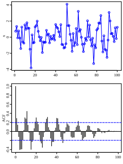
In the analysis of data, a correlogram is a chart of correlation statistics. For example, in time series analysis, a plot of the sample autocorrelations versus is an autocorrelogram. If cross-correlation is plotted, the result is called a cross-correlogram.

Dynamic light scattering (DLS) is a technique in physics that can be used to determine the size distribution profile of small particles in suspension or polymers in solution. In the scope of DLS, temporal fluctuations are usually analyzed by means of the intensity or photon auto-correlation function. In the time domain analysis, the autocorrelation function (ACF) usually decays starting from zero delay time, and faster dynamics due to smaller particles lead to faster decorrelation of scattered intensity trace. It has been shown that the intensity ACF is the Fourier transformation of the power spectrum, and therefore the DLS measurements can be equally well performed in the spectral domain. DLS can also be used to probe the behavior of complex fluids such as concentrated polymer solutions.
Galton's problem, named after Sir Francis Galton, is the problem of drawing inferences from cross-cultural data, due to the statistical phenomenon now called autocorrelation. The problem is now recognized as a general one that applies to all nonexperimental studies and to experimental design as well. It is most simply described as the problem of external dependencies in making statistical estimates when the elements sampled are not statistically independent. Asking two people in the same household whether they watch TV, for example, does not give you statistically independent answers. The sample size, n, for independent observations in this case is one, not two. Once proper adjustments are made that deal with external dependencies, then the axioms of probability theory concerning statistical independence will apply. These axioms are important for deriving measures of variance, for example, or tests of statistical significance.
The Ljung–Box test is a type of statistical test of whether any of a group of autocorrelations of a time series are different from zero. Instead of testing randomness at each distinct lag, it tests the "overall" randomness based on a number of lags, and is therefore a portmanteau test.
In probability theory and statistics, partial correlation measures the degree of association between two random variables, with the effect of a set of controlling random variables removed. If we are interested in finding to what extent there is a numerical relationship between two variables of interest, using their correlation coefficient will give misleading results if there is another, confounding, variable that is numerically related to both variables of interest. This misleading information can be avoided by controlling for the confounding variable, which is done by computing the partial correlation coefficient. This is precisely the motivation for including other right-side variables in a multiple regression; but while multiple regression gives unbiased results for the effect size, it does not give a numerical value of a measure of the strength of the relationship between the two variables of interest.

In time series analysis, the partial autocorrelation function (PACF) gives the partial correlation of a stationary time series with its own lagged values, regressed the values of the time series at all shorter lags. It contrasts with the autocorrelation function, which does not control for other lags.
In statistics, the Breusch–Godfrey test is used to assess the validity of some of the modelling assumptions inherent in applying regression-like models to observed data series. In particular, it tests for the presence of serial correlation that has not been included in a proposed model structure and which, if present, would mean that incorrect conclusions would be drawn from other tests or that sub-optimal estimates of model parameters would be obtained.
A correlation coefficient is a numerical measure of some type of correlation, meaning a statistical relationship between two variables. The variables may be two columns of a given data set of observations, often called a sample, or two components of a multivariate random variable with a known distribution.