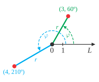
In mathematics, the polar coordinate system is a two-dimensional coordinate system in which each point on a plane is determined by a distance from a reference point and an angle from a reference direction. The reference point is called the pole, and the ray from the pole in the reference direction is the polar axis. The distance from the pole is called the radial coordinate, radial distance or simply radius, and the angle is called the angular coordinate, polar angle, or azimuth. Angles in polar notation are generally expressed in either degrees or radians.

In mathematics, a spherical coordinate system is a coordinate system for three-dimensional space where the position of a given point in space is specified by three numbers, : the radial distance of the radial liner connecting the point to the fixed point of origin ; the polar angle θ of the radial line r; and the azimuthal angle φ of the radial line r.

In mathematics and physics, Laplace's equation is a second-order partial differential equation named after Pierre-Simon Laplace, who first studied its properties. This is often written as

The Navier–Stokes equations are partial differential equations which describe the motion of viscous fluid substances. They were named after French engineer and physicist Claude-Louis Navier and the Irish physicist and mathematician George Gabriel Stokes. They were developed over several decades of progressively building the theories, from 1822 (Navier) to 1842–1850 (Stokes).
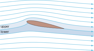
In fluid dynamics, potential flow or irrotational flow refers to a description of a fluid flow with no vorticity in it. Such a description typically arises in the limit of vanishing viscosity, i.e., for an inviscid fluid and with no vorticity present in the flow.
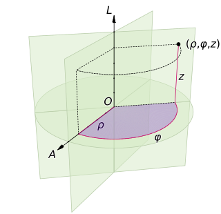
A cylindrical coordinate system is a three-dimensional coordinate system that specifies point positions by the distance from a chosen reference axis (axis L in the image opposite), the direction from the axis relative to a chosen reference direction (axis A), and the distance from a chosen reference plane perpendicular to the axis (plane containing the purple section). The latter distance is given as a positive or negative number depending on which side of the reference plane faces the point.
In vector calculus, the Jacobian matrix of a vector-valued function of several variables is the matrix of all its first-order partial derivatives. When this matrix is square, that is, when the function takes the same number of variables as input as the number of vector components of its output, its determinant is referred to as the Jacobian determinant. Both the matrix and the determinant are often referred to simply as the Jacobian in literature.
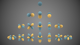
In mathematics and physical science, spherical harmonics are special functions defined on the surface of a sphere. They are often employed in solving partial differential equations in many scientific fields. The table of spherical harmonics contains a list of common spherical harmonics.

In mathematics, the inverse trigonometric functions are the inverse functions of the trigonometric functions. Specifically, they are the inverses of the sine, cosine, tangent, cotangent, secant, and cosecant functions, and are used to obtain an angle from any of the angle's trigonometric ratios. Inverse trigonometric functions are widely used in engineering, navigation, physics, and geometry.
In probability theory, the Borel–Kolmogorov paradox is a paradox relating to conditional probability with respect to an event of probability zero. It is named after Émile Borel and Andrey Kolmogorov.
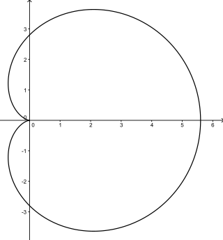
In geometry, a cardioid is a plane curve traced by a point on the perimeter of a circle that is rolling around a fixed circle of the same radius. It can also be defined as an epicycloid having a single cusp. It is also a type of sinusoidal spiral, and an inverse curve of the parabola with the focus as the center of inversion. A cardioid can also be defined as the set of points of reflections of a fixed point on a circle through all tangents to the circle.
This is a list of some vector calculus formulae for working with common curvilinear coordinate systems.
Note: This page uses common physics notation for spherical coordinates, in which is the angle between the z axis and the radius vector connecting the origin to the point in question, while is the angle between the projection of the radius vector onto the x-y plane and the x axis. Several other definitions are in use, and so care must be taken in comparing different sources.

The Stokes parameters are a set of values that describe the polarization state of electromagnetic radiation. They were defined by George Gabriel Stokes in 1852, as a mathematically convenient alternative to the more common description of incoherent or partially polarized radiation in terms of its total intensity (I), (fractional) degree of polarization (p), and the shape parameters of the polarization ellipse. The effect of an optical system on the polarization of light can be determined by constructing the Stokes vector for the input light and applying Mueller calculus, to obtain the Stokes vector of the light leaving the system. The original Stokes paper was discovered independently by Francis Perrin in 1942 and by Subrahamanyan Chandrasekhar in 1947, who named it as the Stokes parameters.
In mathematics, a volume element provides a means for integrating a function with respect to volume in various coordinate systems such as spherical coordinates and cylindrical coordinates. Thus a volume element is an expression of the form

In mathematics (specifically multivariable calculus), a multiple integral is a definite integral of a function of several real variables, for instance, f(x, y) or f(x, y, z). Physical (natural philosophy) interpretation: S any surface, V any volume, etc.. Incl. variable to time, position, etc.
In physics and mathematics, the solid harmonics are solutions of the Laplace equation in spherical polar coordinates, assumed to be (smooth) functions . There are two kinds: the regular solid harmonics, which are well-defined at the origin and the irregular solid harmonics, which are singular at the origin. Both sets of functions play an important role in potential theory, and are obtained by rescaling spherical harmonics appropriately:
In mathematics, vector spherical harmonics (VSH) are an extension of the scalar spherical harmonics for use with vector fields. The components of the VSH are complex-valued functions expressed in the spherical coordinate basis vectors.
In fluid dynamics, the Oseen equations describe the flow of a viscous and incompressible fluid at small Reynolds numbers, as formulated by Carl Wilhelm Oseen in 1910. Oseen flow is an improved description of these flows, as compared to Stokes flow, with the (partial) inclusion of convective acceleration.


