Log-polar coordinates

Last updated

In mathematics, log-polar coordinates (or logarithmic polar coordinates) is a coordinate system in two dimensions, where a point is identified by two numbers, one for the logarithm of the distance to a certain point, and one for an angle. Log-polar coordinates are closely connected to polar coordinates, which are usually used to describe domains in the plane with some sort of rotational symmetry. In areas like harmonic and complex analysis, the log-polar coordinates are more canonical than polar coordinates.

Contents

Definition and coordinate transformations

Log-polar coordinates in the plane consist of a pair of real numbers (ρ,θ), where ρ is the logarithm of the distance between a given point and the origin and θ is the angle between a line of reference (the x-axis) and the line through the origin and the point. The angular coordinate is the same as for polar coordinates, while the radial coordinate is transformed according to the rule

.

where is the distance to the origin. The formulas for transformation from Cartesian coordinates to log-polar coordinates are given by

and the formulas for transformation from log-polar to Cartesian coordinates are

By using complex numbers (x, y) = x + iy, the latter transformation can be written as

i.e. the complex exponential function. From this follows that basic equations in harmonic and complex analysis will have the same simple form as in Cartesian coordinates. This is not the case for polar coordinates.

Some important equations in log-polar coordinates

Laplace's equation

Laplace's equation in two dimensions is given by

in Cartesian coordinates. Writing the same equation in polar coordinates gives the more complicated equation

or equivalently

However, from the relation it follows that so Laplace's equation in log-polar coordinates,

has the same simple expression as in Cartesian coordinates. This is true for all coordinate systems where the transformation to Cartesian coordinates is given by a conformal mapping. Thus, when considering Laplace's equation for a part of the plane with rotational symmetry, e.g. a circular disk, log-polar coordinates is the natural choice.

CauchyRiemann equations

A similar situation arises when considering analytical functions. An analytical function written in Cartesian coordinates satisfies the CauchyRiemann equations:

If the function instead is expressed in polar form , the CauchyRiemann equations take the more complicated form

Just as in the case with Laplace's equation, the simple form of Cartesian coordinates is recovered by changing polar into log-polar coordinates (let ):

The CauchyRiemann equations can also be written in one single equation as

By expressing and in terms of and this equation can be written in the equivalent form

Euler's equation

When one wants to solve the Dirichlet problem in a domain with rotational symmetry, the usual thing to do is to use the method of separation of variables for partial differential equations for Laplace's equation in polar form. This means that you write . Laplace's equation is then separated into two ordinary differential equations

where is a constant. The first of these has constant coefficients and is easily solved. The second is a special case of Euler's equation

where are constants. This equation is usually solved by the ansatz , but through use of log-polar radius, it can be changed into an equation with constant coefficients:

When considering Laplace's equation, and so the equation for takes the simple form

When solving the Dirichlet problem in Cartesian coordinates, these are exactly the equations for and . Thus, once again the natural choice for a domain with rotational symmetry is not polar, but rather log-polar, coordinates.

Discrete geometry

Discrete coordinate system in a circular disc given by log-polar coordinates (n = 25) Logpolargrid.jpg
Discrete coordinate system in a circular disc given by log-polar coordinates (n = 25)
Discrete coordinate system in a circular disc that can easily be expressed in log-polar coordinates (n = 25) Logspiralgrid.png
Discrete coordinate system in a circular disc that can easily be expressed in log-polar coordinates (n = 25)
Part of a Mandelbrot fractal showing spiral behaviour Mandelbrotzoom1.jpg
Part of a Mandelbrot fractal showing spiral behaviour

In order to solve a PDE numerically in a domain, a discrete coordinate system must be introduced in this domain. If the domain has rotational symmetry and you want a grid consisting of rectangles, polar coordinates are a poor choice, since in the center of the circle it gives rise to triangles rather than rectangles. However, this can be remedied by introducing log-polar coordinates in the following way. Divide the plane into a grid of squares with side length 2/n, where n is a positive integer. Use the complex exponential function to create a log-polar grid in the plane. The left half-plane is then mapped onto the unit disc, with the number of radii equal to n. It can be even more advantageous to instead map the diagonals in these squares, which gives a discrete coordinate system in the unit disc consisting of spirals, see the figure to the right.

Dirichlet-to-Neumann operator

The latter coordinate system is for instance suitable for dealing with Dirichlet and Neumann problems. If the discrete coordinate system is interpreted as an undirected graph in the unit disc, it can be considered as a model for an electrical network. To every line segment in the graph is associated a conductance given by a function . The electrical network will then serve as a discrete model for the Dirichlet problem in the unit disc, where the Laplace equation takes the form of Kirchhoff's law. On the nodes on the boundary of the circle, an electrical potential (Dirichlet data) is defined, which induces an electric current (Neumann data) through the boundary nodes. The linear operator from Dirichlet data to Neumann data is called a Dirichlet-to-Neumann operator, and depends on the topology and conductance of the network.

In the case with the continuous disc, it follows that if the conductance is homogeneous, let's say everywhere, then the Dirichlet-to-Neumann operator satisfies the following equation

In order to get a good discrete model of the Dirichlet problem, it would be useful to find a graph in the unit disc whose (discrete) Dirichlet-to-Neumann operator has the same property. Even though polar coordinates don't give us any answer, this is approximate/asymptotically, what the rotationally symmetric network given by log-polar coordinates provides us with. [1]

Image analysis

Already at the end of the 1970s, applications for the discrete spiral coordinate system were given in image analysis ( image registration ) . To represent an image in this coordinate system rather than in Cartesian coordinates, gives computational advantages when rotating or zooming in an image. Also, the photo receptors in the retina in the human eye are distributed in a way that has big similarities with the spiral coordinate system. [2] It can also be found in the Mandelbrot fractal (see picture to the right).

Log-polar coordinates can also be used to construct fast methods for the Radon transform and its inverse. [3]

See also

Related Research Articles

A centripetal force is a force that makes a body follow a curved path. Its direction is always orthogonal to the motion of the body and towards the fixed point of the instantaneous center of curvature of the path. Isaac Newton described it as "a force by which bodies are drawn or impelled, or in any way tend, towards a point as to a centre". In Newtonian mechanics, gravity provides the centripetal force causing astronomical orbits.

<span class="mw-page-title-main">Polar coordinate system</span> Coordinates determined by distance and angle

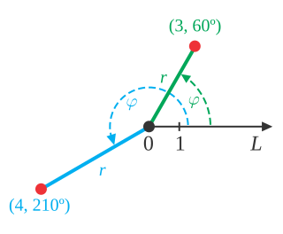
In mathematics, the polar coordinate system is a two-dimensional coordinate system in which each point on a plane is determined by a distance from a reference point and an angle from a reference direction. The reference point is called the pole, and the ray from the pole in the reference direction is the polar axis. The distance from the pole is called the radial coordinate, radial distance or simply radius, and the angle is called the angular coordinate, polar angle, or azimuth. Angles in polar notation are generally expressed in either degrees or radians.

Spherical coordinate system 3-dimensional coordinate system

In mathematics, a spherical coordinate system is a coordinate system for three-dimensional space where the position of a point is specified by three numbers: the radial distance of that point from a fixed origin, its polar angle measured from a fixed zenith direction, and the azimuthal angle of its orthogonal projection on a reference plane that passes through the origin and is orthogonal to the zenith, measured from a fixed reference direction on that plane. It can be seen as the three-dimensional version of the polar coordinate system.

<span class="mw-page-title-main">Laplace's equation</span> Second order partial differential equation

In mathematics and physics, Laplace's equation is a second-order partial differential equation named after Pierre-Simon Laplace, who first studied its properties. This is often written as

<span class="mw-page-title-main">Navier–Stokes equations</span> Equations describing the motion of viscous fluid substances

In physics, the Navier–Stokes equations are certain partial differential equations which describe the motion of viscous fluid substances, named after French engineer and physicist Claude-Louis Navier and Anglo-Irish physicist and mathematician George Gabriel Stokes. They were developed over several decades of progressively building the theories, from 1822 (Navier) to 1842–1850 (Stokes).

<span class="mw-page-title-main">Potential flow</span> Velocity field as the gradient of a scalar function

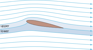
In fluid dynamics, potential flow describes the velocity field as the gradient of a scalar function: the velocity potential. As a result, a potential flow is characterized by an irrotational velocity field, which is a valid approximation for several applications. The irrotationality of a potential flow is due to the curl of the gradient of a scalar always being equal to zero.

Unit vector Vector of length one

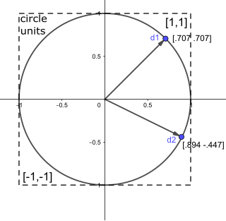
In mathematics, a unit vector in a normed vector space is a vector of length 1. A unit vector is often denoted by a lowercase letter with a circumflex, or "hat", as in .

In mathematics, the Laplace operator or Laplacian is a differential operator given by the divergence of the gradient of a scalar function on Euclidean space. It is usually denoted by the symbols , , or . In a Cartesian coordinate system, the Laplacian is given by the sum of second partial derivatives of the function with respect to each independent variable. In other coordinate systems, such as cylindrical and spherical coordinates, the Laplacian also has a useful form. Informally, the Laplacian Δf (p) of a function f at a point p measures by how much the average value of f over small spheres or balls centered at p deviates from f (p).

<span class="mw-page-title-main">Cylindrical coordinate system</span> 3-dimensional coordinate system

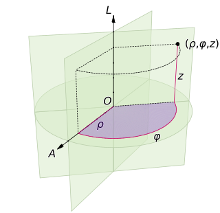
A cylindrical coordinate system is a three-dimensional coordinate system that specifies point positions by the distance from a chosen reference axis (axis L in the image opposite), the direction from the axis relative to a chosen reference direction (axis A), and the distance from a chosen reference plane perpendicular to the axis (plane containing the purple section). The latter distance is given as a positive or negative number depending on which side of the reference plane faces the point.

Linear elasticity is a mathematical model of how solid objects deform and become internally stressed due to prescribed loading conditions. It is a simplification of the more general nonlinear theory of elasticity and a branch of continuum mechanics.

This is a list of some vector calculus formulae for working with common curvilinear coordinate systems.

In mathematics, a Killing vector field, named after Wilhelm Killing, is a vector field on a Riemannian manifold that preserves the metric. Killing fields are the infinitesimal generators of isometries; that is, flows generated by Killing fields are continuous isometries of the manifold. More simply, the flow generates a symmetry, in the sense that moving each point of an object the same distance in the direction of the Killing vector will not distort distances on the object.

In gas dynamics, Chaplygin's equation, named after Sergei Alekseevich Chaplygin (1902), is a partial differential equation useful in the study of transonic flow. It is

Helmholtz equation Eigenvalue problem for the Laplace operator

In mathematics, the eigenvalue problem for the Laplace operator is known as the Helmholtz equation. It corresponds to the linear partial differential equation

In general relativity, the metric tensor is the fundamental object of study. It may loosely be thought of as a generalization of the gravitational potential of Newtonian gravitation. The metric captures all the geometric and causal structure of spacetime, being used to define notions such as time, distance, volume, curvature, angle, and separation of the future and the past.

In Newton's theory of gravitation and in various relativistic classical theories of gravitation, such as general relativity, the tidal tensor represents

  1. tidal accelerations of a cloud of test particles,
  2. tidal stresses in a small object immersed in an ambient gravitational field.

In physics and fluid mechanics, a Blasius boundary layer describes the steady two-dimensional laminar boundary layer that forms on a semi-infinite plate which is held parallel to a constant unidirectional flow. Falkner and Skan later generalized Blasius' solution to wedge flow, i.e. flows in which the plate is not parallel to the flow.

In fluid dynamics, the Oseen equations describe the flow of a viscous and incompressible fluid at small Reynolds numbers, as formulated by Carl Wilhelm Oseen in 1910. Oseen flow is an improved description of these flows, as compared to Stokes flow, with the (partial) inclusion of convective acceleration.

Potential flow around a circular cylinder Classical solution for inviscid, incompressible flow around a cyclinder

In mathematics, potential flow around a circular cylinder is a classical solution for the flow of an inviscid, incompressible fluid around a cylinder that is transverse to the flow. Far from the cylinder, the flow is unidirectional and uniform. The flow has no vorticity and thus the velocity field is irrotational and can be modeled as a potential flow. Unlike a real fluid, this solution indicates a net zero drag on the body, a result known as d'Alembert's paradox.

References

  1. [ dead link ]
  2. Weiman, Chaikin, Logarithmic Spiral Grids for Image Processing and Display, Computer Graphics and Image Processing 11, 197226 (1979).
  3. Andersson, Fredrik, Fast Inversion of the Radon Transform Using Log-polar Coordinates and Partial Back-Projections, SIAM J. Appl. Math. 65, 818837 (2005).