
In statistical mechanics and information theory, the Fokker–Planck equation is a partial differential equation that describes the time evolution of the probability density function of the velocity of a particle under the influence of drag forces and random forces, as in Brownian motion. The equation can be generalized to other observables as well. The Fokker-Planck equation has multiple applications in information theory, graph theory, data science, finance, economics etc.

The path integral formulation is a description in quantum mechanics that generalizes the stationary action principle of classical mechanics. It replaces the classical notion of a single, unique classical trajectory for a system with a sum, or functional integral, over an infinity of quantum-mechanically possible trajectories to compute a quantum amplitude.
In information geometry, the Fisher information metric is a particular Riemannian metric which can be defined on a smooth statistical manifold, i.e., a smooth manifold whose points are probability measures defined on a common probability space. It can be used to calculate the informational difference between measurements.

A Boltzmann machine is a stochastic spin-glass model with an external field, i.e., a Sherrington–Kirkpatrick model, that is a stochastic Ising model. It is a statistical physics technique applied in the context of cognitive science. It is also classified as a Markov random field.
In the domain of physics and probability, a Markov random field (MRF), Markov network or undirected graphical model is a set of random variables having a Markov property described by an undirected graph. In other words, a random field is said to be a Markov random field if it satisfies Markov properties. The concept originates from the Sherrington–Kirkpatrick model.

As a machine-learning algorithm, backpropagation performs a backward pass to adjust a neural network model's parameters, aiming to minimize error. In a multi-layered network, backpropagation uses the following steps:
- Propagate training data through the model from input to predicted output by computing the successive hidden layers' outputs and finally the final layer's output.
- Adjust the model weights to reduce the error relative to the weights.
- The error is typically the squared difference between prediction and target.
- For each weight, the slope or derivative of the error is found, and the weight adjusted by a negative multiple of this derivative, so as to go downslope toward the minimum-error configuration.
- This derivative is easy to calculate for final layer weights, and possible to calculate for one layer given the next layer's derivatives. Starting at the end, then, the derivatives are calculated layer by layer toward the beginning -- thus "backpropagation".
- Repeatedly update the weights until they converge or the model has undergone enough iterations.
In the study of graphs and networks, the degree of a node in a network is the number of connections it has to other nodes and the degree distribution is the probability distribution of these degrees over the whole network.
The birth–death process is a special case of continuous-time Markov process where the state transitions are of only two types: "births", which increase the state variable by one and "deaths", which decrease the state by one. It was introduced by William Feller. The model's name comes from a common application, the use of such models to represent the current size of a population where the transitions are literal births and deaths. Birth–death processes have many applications in demography, queueing theory, performance engineering, epidemiology, biology and other areas. They may be used, for example, to study the evolution of bacteria, the number of people with a disease within a population, or the number of customers in line at the supermarket.
In queueing theory, a discipline within the mathematical theory of probability, a Jackson network is a class of queueing network where the equilibrium distribution is particularly simple to compute as the network has a product-form solution. It was the first significant development in the theory of networks of queues, and generalising and applying the ideas of the theorem to search for similar product-form solutions in other networks has been the subject of much research, including ideas used in the development of the Internet. The networks were first identified by James R. Jackson and his paper was re-printed in the journal Management Science’s ‘Ten Most Influential Titles of Management Sciences First Fifty Years.’
The Watts–Strogatz model is a random graph generation model that produces graphs with small-world properties, including short average path lengths and high clustering. It was proposed by Duncan J. Watts and Steven Strogatz in their article published in 1998 in the Nature scientific journal. The model also became known as the (Watts) beta model after Watts used to formulate it in his popular science book Six Degrees.

The Gaussian network model (GNM) is a representation of a biological macromolecule as an elastic mass-and-spring network to study, understand, and characterize the mechanical aspects of its long-time large-scale dynamics. The model has a wide range of applications from small proteins such as enzymes composed of a single domain, to large macromolecular assemblies such as a ribosome or a viral capsid. Protein domain dynamics plays key roles in a multitude of molecular recognition and cell signalling processes. Protein domains, connected by intrinsically disordered flexible linker domains, induce long-range allostery via protein domain dynamics. The resultant dynamic modes cannot be generally predicted from static structures of either the entire protein or individual domains.
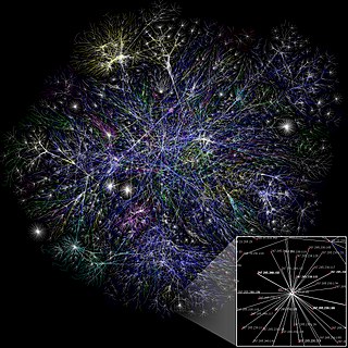
Network science is an academic field which studies complex networks such as telecommunication networks, computer networks, biological networks, cognitive and semantic networks, and social networks, considering distinct elements or actors represented by nodes and the connections between the elements or actors as links. The field draws on theories and methods including graph theory from mathematics, statistical mechanics from physics, data mining and information visualization from computer science, inferential modeling from statistics, and social structure from sociology. The United States National Research Council defines network science as "the study of network representations of physical, biological, and social phenomena leading to predictive models of these phenomena."
In fracture mechanics, the energy release rate, , is the rate at which energy is transformed as a material undergoes fracture. Mathematically, the energy release rate is expressed as the decrease in total potential energy per increase in fracture surface area, and is thus expressed in terms of energy per unit area. Various energy balances can be constructed relating the energy released during fracture to the energy of the resulting new surface, as well as other dissipative processes such as plasticity and heat generation. The energy release rate is central to the field of fracture mechanics when solving problems and estimating material properties related to fracture and fatigue.

Diffusion is the net movement of anything generally from a region of higher concentration to a region of lower concentration. Diffusion is driven by a gradient in Gibbs free energy or chemical potential. It is possible to diffuse "uphill" from a region of lower concentration to a region of higher concentration, as in spinodal decomposition. Diffusion is a stochastic process due to the inherent randomness of the diffusing entity and can be used to model many real-life stochastic scenarios. Therefore, diffusion and the corresponding mathematical models are used in several fields beyond physics, such as statistics, probability theory, information theory, neural networks, finance, and marketing.
Simultaneous perturbation stochastic approximation (SPSA) is an algorithmic method for optimizing systems with multiple unknown parameters. It is a type of stochastic approximation algorithm. As an optimization method, it is appropriately suited to large-scale population models, adaptive modeling, simulation optimization, and atmospheric modeling. Many examples are presented at the SPSA website http://www.jhuapl.edu/SPSA. A comprehensive book on the subject is Bhatnagar et al. (2013). An early paper on the subject is Spall (1987) and the foundational paper providing the key theory and justification is Spall (1992).
The Louvain method for community detection is a method to extract non-overlapping communities from large networks created by Blondel et al. from the University of Louvain. The method is a greedy optimization method that appears to run in time where is the number of nodes in the network.
A two-dimensional conformal field theory is a quantum field theory on a Euclidean two-dimensional space, that is invariant under local conformal transformations.

In network science, the configuration model is a method for generating random networks from a given degree sequence. It is widely used as a reference model for real-life social networks, because it allows the modeler to incorporate arbitrary degree distributions.

The hyperbolastic functions, also known as hyperbolastic growth models, are mathematical functions that are used in medical statistical modeling. These models were originally developed to capture the growth dynamics of multicellular tumor spheres, and were introduced in 2005 by Mohammad Tabatabai, David Williams, and Zoran Bursac. The precision of hyperbolastic functions in modeling real world problems is somewhat due to their flexibility in their point of inflection. These functions can be used in a wide variety of modeling problems such as tumor growth, stem cell proliferation, pharma kinetics, cancer growth, sigmoid activation function in neural networks, and epidemiological disease progression or regression.
In computational and mathematical biology, a biological lattice-gas cellular automaton (BIO-LGCA) is a discrete model for moving and interacting biological agents, a type of cellular automaton. The BIO-LGCA is based on the lattice-gas cellular automaton (LGCA) model used in fluid dynamics. A BIO-LGCA model describes cells and other motile biological agents as point particles moving on a discrete lattice, thereby interacting with nearby particles. Contrary to classic cellular automaton models, particles in BIO-LGCA are defined by their position and velocity. This allows to model and analyze active fluids and collective migration mediated primarily through changes in momentum, rather than density. BIO-LGCA applications include cancer invasion and cancer progression.


