In statistics, the likelihood-ratio test assesses the goodness of fit of two competing statistical models, specifically one found by maximization over the entire parameter space and another found after imposing some constraint, based on the ratio of their likelihoods. If the constraint is supported by the observed data, the two likelihoods should not differ by more than sampling error. Thus the likelihood-ratio test tests whether this ratio is significantly different from one, or equivalently whether its natural logarithm is significantly different from zero.

In probability theory and statistics, the exponential distribution or negative exponential distribution is the probability distribution of the time between events in a Poisson point process, i.e., a process in which events occur continuously and independently at a constant average rate. It is a particular case of the gamma distribution. It is the continuous analogue of the geometric distribution, and it has the key property of being memoryless. In addition to being used for the analysis of Poisson point processes it is found in various other contexts.

In probability theory and statistics, the Weibull distribution is a continuous probability distribution. It models a broad range of random variables, largely in the nature of a time to failure or time between events. Examples are maximum one-day rainfalls and the time a user spends on a web page.

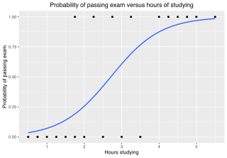
In statistics, the logistic model is a statistical model that models the probability of an event taking place by having the log-odds for the event be a linear combination of one or more independent variables. In regression analysis, logistic regression is estimating the parameters of a logistic model. Formally, in binary logistic regression there is a single binary dependent variable, coded by an indicator variable, where the two values are labeled "0" and "1", while the independent variables can each be a binary variable or a continuous variable. The corresponding probability of the value labeled "1" can vary between 0 and 1, hence the labeling; the function that converts log-odds to probability is the logistic function, hence the name. The unit of measurement for the log-odds scale is called a logit, from logistic unit, hence the alternative names. See § Background and § Definition for formal mathematics, and § Example for a worked example.
Pearson's chi-squared test is a statistical test applied to sets of categorical data to evaluate how likely it is that any observed difference between the sets arose by chance. It is the most widely used of many chi-squared tests – statistical procedures whose results are evaluated by reference to the chi-squared distribution. Its properties were first investigated by Karl Pearson in 1900. In contexts where it is important to improve a distinction between the test statistic and its distribution, names similar to Pearson χ-squared test or statistic are used.
Survival analysis is a branch of statistics for analyzing the expected duration of time until one event occurs, such as death in biological organisms and failure in mechanical systems. This topic is called reliability theory or reliability analysis in engineering, duration analysis or duration modelling in economics, and event history analysis in sociology. Survival analysis attempts to answer certain questions, such as what is the proportion of a population which will survive past a certain time? Of those that survive, at what rate will they die or fail? Can multiple causes of death or failure be taken into account? How do particular circumstances or characteristics increase or decrease the probability of survival?
In statistics, G-tests are likelihood-ratio or maximum likelihood statistical significance tests that are increasingly being used in situations where chi-squared tests were previously recommended.

Trip distribution is the second component in the traditional four-step transportation forecasting model. This step matches tripmakers’ origins and destinations to develop a “trip table”, a matrix that displays the number of trips going from each origin to each destination. Historically, this component has been the least developed component of the transportation planning model.
In statistics, the Vuong closeness test is a likelihood-ratio-based test for model selection using the Kullback–Leibler information criterion. This statistic makes probabilistic statements about two models. They can be nested, strictly non-nested or partially non-nested. The statistic tests the null hypothesis that the two models are equally close to the true data generating process, against the alternative that one model is closer. It cannot make any decision whether the "closer" model is the true model.
The goodness of fit of a statistical model describes how well it fits a set of observations. Measures of goodness of fit typically summarize the discrepancy between observed values and the values expected under the model in question. Such measures can be used in statistical hypothesis testing, e.g. to test for normality of residuals, to test whether two samples are drawn from identical distributions, or whether outcome frequencies follow a specified distribution. In the analysis of variance, one of the components into which the variance is partitioned may be a lack-of-fit sum of squares.
In statistics, a generalized additive model (GAM) is a generalized linear model in which the linear response variable depends linearly on unknown smooth functions of some predictor variables, and interest focuses on inference about these smooth functions.
Proportional hazards models are a class of survival models in statistics. Survival models relate the time that passes, before some event occurs, to one or more covariates that may be associated with that quantity of time. In a proportional hazards model, the unique effect of a unit increase in a covariate is multiplicative with respect to the hazard rate. For example, taking a drug may halve one's hazard rate for a stroke occurring, or, changing the material from which a manufactured component is constructed may double its hazard rate for failure. Other types of survival models such as accelerated failure time models do not exhibit proportional hazards. The accelerated failure time model describes a situation where the biological or mechanical life history of an event is accelerated.
Omnibus tests are a kind of statistical test. They test whether the explained variance in a set of data is significantly greater than the unexplained variance, overall. One example is the F-test in the analysis of variance. There can be legitimate significant effects within a model even if the omnibus test is not significant. For instance, in a model with two independent variables, if only one variable exerts a significant effect on the dependent variable and the other does not, then the omnibus test may be non-significant. This fact does not affect the conclusions that may be drawn from the one significant variable. In order to test effects within an omnibus test, researchers often use contrasts.
In statistics, a power transform is a family of functions applied to create a monotonic transformation of data using power functions. It is a data transformation technique used to stabilize variance, make the data more normal distribution-like, improve the validity of measures of association, and for other data stabilization procedures.
In statistics, confirmatory factor analysis (CFA) is a special form of factor analysis, most commonly used in social science research. It is used to test whether measures of a construct are consistent with a researcher's understanding of the nature of that construct. As such, the objective of confirmatory factor analysis is to test whether the data fit a hypothesized measurement model. This hypothesized model is based on theory and/or previous analytic research. CFA was first developed by Jöreskog (1969) and has built upon and replaced older methods of analyzing construct validity such as the MTMM Matrix as described in Campbell & Fiske (1959).
The logrank test, or log-rank test, is a hypothesis test to compare the survival distributions of two samples. It is a nonparametric test and appropriate to use when the data are right skewed and censored. It is widely used in clinical trials to establish the efficacy of a new treatment in comparison with a control treatment when the measurement is the time to event. The test is sometimes called the Mantel–Cox test. The logrank test can also be viewed as a time-stratified Cochran–Mantel–Haenszel test.

In probability theory and statistics, the Conway–Maxwell–Poisson distribution is a discrete probability distribution named after Richard W. Conway, William L. Maxwell, and Siméon Denis Poisson that generalizes the Poisson distribution by adding a parameter to model overdispersion and underdispersion. It is a member of the exponential family, has the Poisson distribution and geometric distribution as special cases and the Bernoulli distribution as a limiting case.
In statistics, Tukey's test of additivity, named for John Tukey, is an approach used in two-way ANOVA to assess whether the factor variables are additively related to the expected value of the response variable. It can be applied when there are no replicated values in the data set, a situation in which it is impossible to directly estimate a fully general non-additive regression structure and still have information left to estimate the error variance. The test statistic proposed by Tukey has one degree of freedom under the null hypothesis, hence this is often called "Tukey's one-degree-of-freedom test."
In statistics Wilks' theorem offers an asymptotic distribution of the log-likelihood ratio statistic, which can be used to produce confidence intervals for maximum-likelihood estimates or as a test statistic for performing the likelihood-ratio test.
In statistics, the variance function is a smooth function which depicts the variance of a random quantity as a function of its mean. The variance function is a measure of heteroscedasticity and plays a large role in many settings of statistical modelling. It is a main ingredient in the generalized linear model framework and a tool used in non-parametric regression, semiparametric regression and functional data analysis. In parametric modeling, variance functions take on a parametric form and explicitly describe the relationship between the variance and the mean of a random quantity. In a non-parametric setting, the variance function is assumed to be a smooth function.


