In mathematics, the Laplace transform, named after its inventor Pierre-Simon Laplace, is an integral transform that converts a function of a real variable to a function of a complex variable . The transform has many applications in science and engineering because it is a tool for solving differential equations. In particular, it transforms linear differential equations into algebraic equations and convolution into multiplication.
In the mathematical field of dynamical systems, an attractor is a set of states toward which a system tends to evolve, for a wide variety of starting conditions of the system. System values that get close enough to the attractor values remain close even if slightly disturbed.

A geometric Brownian motion (GBM) is a continuous-time stochastic process in which the logarithm of the randomly varying quantity follows a Brownian motion with drift. It is an important example of stochastic processes satisfying a stochastic differential equation (SDE); in particular, it is used in mathematical finance to model stock prices in the Black–Scholes model.
In mathematics, an autonomous system or autonomous differential equation is a system of ordinary differential equations which does not explicitly depend on the independent variable. When the variable is time, they are also called time-invariant systems.
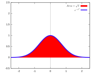
The Gaussian integral, also known as the Euler–Poisson integral, is the integral of the Gaussian function over the entire real line. Named after the German mathematician Carl Friedrich Gauss, the integral is
Model predictive control (MPC) is an advanced method of process control that is used to control a process while satisfying a set of constraints. It has been in use in the process industries in chemical plants and oil refineries since the 1980s. In recent years it has also been used in power system balancing models and in power electronics. Model predictive controllers rely on dynamic models of the process, most often linear empirical models obtained by system identification. The main advantage of MPC is the fact that it allows the current timeslot to be optimized, while keeping future timeslots in account. This is achieved by optimizing a finite time-horizon, but only implementing the current timeslot and then optimizing again, repeatedly, thus differing from a linear–quadratic regulator (LQR). Also MPC has the ability to anticipate future events and can take control actions accordingly. PID controllers do not have this predictive ability. MPC is nearly universally implemented as a digital control, although there is research into achieving faster response times with specially designed analog circuitry.

In mathematics, there are several integrals known as the Dirichlet integral, after the German mathematician Peter Gustav Lejeune Dirichlet, one of which is the improper integral of the sinc function over the positive real line:

The Rössler attractor is the attractor for the Rössler system, a system of three non-linear ordinary differential equations originally studied by Otto Rössler in the 1970s. These differential equations define a continuous-time dynamical system that exhibits chaotic dynamics associated with the fractal properties of the attractor.

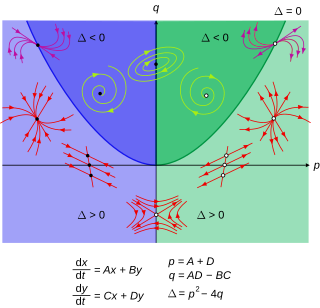
In applied mathematics, in particular the context of nonlinear system analysis, a phase plane is a visual display of certain characteristics of certain kinds of differential equations; a coordinate plane with axes being the values of the two state variables, say, or etc.. It is a two-dimensional case of the general n-dimensional phase space.
In calculus, the Leibniz integral rule for differentiation under the integral sign, named after Gottfried Leibniz, states that for an integral of the form

In physics and mathematics, the Ikeda map is a discrete-time dynamical system given by the complex map

The Lorenz system is a system of ordinary differential equations first studied by mathematician and meteorologist Edward Lorenz. It is notable for having chaotic solutions for certain parameter values and initial conditions. In particular, the Lorenz attractor is a set of chaotic solutions of the Lorenz system. In popular media the "butterfly effect" stems from the real-world implications of the Lorenz attractor, i.e. that in any physical system, in the absence of perfect knowledge of the initial conditions, our ability to predict its future course will always fail. This underscores that physical systems can be completely deterministic and yet still be inherently unpredictable even in the absence of quantum effects. The shape of the Lorenz attractor itself, when plotted graphically, may also be seen to resemble a butterfly.
In Itô calculus, the Euler–Maruyama method is a method for the approximate numerical solution of a stochastic differential equation (SDE). It is an extension of the Euler method for ordinary differential equations to stochastic differential equations. It is named after Leonhard Euler and Gisiro Maruyama. Unfortunately, the same generalization cannot be done for any arbitrary deterministic method.
In mathematics, the Milstein method is a technique for the approximate numerical solution of a stochastic differential equation. It is named after Grigori N. Milstein who first published the method in 1974.
The PROPT MATLAB Optimal Control Software is a new generation platform for solving applied optimal control and parameters estimation problems.
In mathematics, the slow manifold of an equilibrium point of a dynamical system occurs as the most common example of a center manifold. One of the main methods of simplifying dynamical systems, is to reduce the dimension of the system to that of the slow manifold—center manifold theory rigorously justifies the modelling. For example, some global and regional models of the atmosphere or oceans resolve the so-called quasi-geostrophic flow dynamics on the slow manifold of the atmosphere/oceanic dynamics, and is thus crucial to forecasting with a climate model.
In dynamical systems, a branch of mathematics, an invariant manifold is a topological manifold that is invariant under the action of the dynamical system. Examples include the slow manifold, center manifold, stable manifold, unstable manifold, subcenter manifold and inertial manifold.

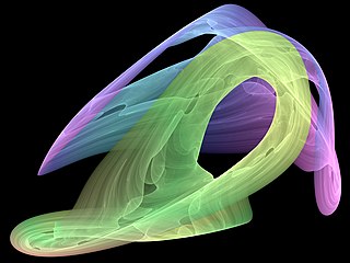
In the mathematics of dynamical systems, the double-scroll attractor is a strange attractor observed from a physical electronic chaotic circuit with a single nonlinear resistor. The double-scroll system is often described by a system of three nonlinear ordinary differential equations and a 3-segment piecewise-linear equation. This makes the system easily simulated numerically and easily manifested physically due to Chua's circuits' simple design.
The GEKKO Python package solves large-scale mixed-integer and differential algebraic equations with nonlinear programming solvers. Modes of operation include machine learning, data reconciliation, real-time optimization, dynamic simulation, and nonlinear model predictive control. In addition, the package solves Linear programming (LP), Quadratic programming (QP), Quadratically constrained quadratic program (QCQP), Nonlinear programming (NLP), Mixed integer programming (MIP), and Mixed integer linear programming (MILP). GEKKO is available in Python and installed with pip from PyPI of the Python Software Foundation.

In dynamical systems, a spectral submanifold (SSM) is the unique smoothest invariant manifold serving as the nonlinear extension of a spectral subspace of a linear dynamical system under the addition of nonlinearities. SSM theory provides conditions for when invariant properties of eigenspaces of a linear dynamical system can be extended to a nonlinear system, and therefore motivates the use of SSMs in nonlinear dimensionality reduction.


