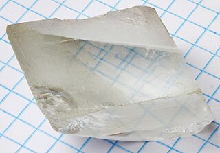
Direction dependence of magnetization in a crystal
In physics, a ferromagnetic material is said to have magnetocrystalline anisotropy if it takes more energy to magnetize it in certain directions than in others. These directions are usually related to the principal axes of its crystal lattice. It is a special case of magnetic anisotropy. In other words, the excess energy required to magnetize a specimen in a particular direction over that required to magnetize it along the easy direction is called crystalline anisotropy energy.
The spin-orbit interaction is the primary source of magnetocrystalline anisotropy. It is basically the orbital motion of the electrons which couples with crystal electric field giving rise to the first order contribution to magnetocrystalline anisotropy. The second order arises due to the mutual interaction of the magnetic dipoles. This effect is weak compared to the exchange interaction and is difficult to compute from first principles, although some successful computations have been made.[1]
Practical relevance
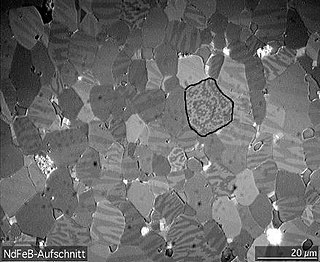
Magnetocrystalline anisotropy has a great influence on industrial uses of ferromagnetic materials. Materials with high magnetic anisotropy usually have high coercivity, that is, they are hard to demagnetize. These are called "hard" ferromagnetic materials and are used to make permanent magnets. For example, the high anisotropy of rare-earth metals is mainly responsible for the strength of rare-earth magnets. During manufacture of magnets, a powerful magnetic field aligns the microcrystalline grains of the metal such that their "easy" axes of magnetization all point in the same direction, freezing a strong magnetic field into the material.
On the other hand, materials with low magnetic anisotropy usually have low coercivity, their magnetization is easy to change. These are called "soft" ferromagnets and are used to make magnetic cores for transformers and inductors. The small energy required to turn the direction of magnetization minimizes core losses, energy dissipated in the transformer core when the alternating current changes direction.
Thermodynamic theory
The magnetocrystalline anisotropy energy is generally represented as an expansion in powers of the direction cosines of the magnetization. The magnetization vector can be written M = Ms(α,β,γ), where Ms is the saturation magnetization. Because of time reversal symmetry, only even powers of the cosines are allowed.[2] The nonzero terms in the expansion depend on the crystal system (e.g., cubic or hexagonal).[2] The order of a term in the expansion is the sum of all the exponents of magnetization components, e.g., αβ is second order.
Examples of easy and hard directions: Although easy directions often (not always ) coincide with crystallographic axes of symmetry, it is important to note that there is no way of predicting easy directions from crystal structure alone.
Uniaxial anisotropy
Uniaxial anisotropy energy plotted for 2D case. The magnetization direction is constrained to vary on a circle and the energy takes different values with the minima indicated by the vectors in red.
More than one kind of crystal system has a single axis of high symmetry (threefold, fourfold or sixfold). The anisotropy of such crystals is called uniaxial anisotropy. If the z axis is taken to be the main symmetry axis of the crystal, the lowest order term in the energy is[5]
The ratio E/V is an energy density (energy per unit volume). This can also be represented in spherical polar coordinates with α = cos sin θ, β = sin sin θ, and γ = cos θ:
The parameter K1, often represented as Ku, has units of energy density and depends on composition and temperature.
The minima in this energy with respect to θ satisfy
If K1> 0, the directions of lowest energy are the ±z directions. The z axis is called the easy axis. If K1< 0, there is an easy plane perpendicular to the symmetry axis (the basal plane of the crystal).
Many models of magnetization represent the anisotropy as uniaxial and ignore higher order terms. However, if K1< 0, the lowest energy term does not determine the direction of the easy axes within the basal plane. For this, higher-order terms are needed, and these depend on the crystal system (hexagonal, tetragonal or rhombohedral).[2]
The hexagonal lattice cell.
The tetragonal lattice cell.
The rhombohedral lattice cell.
Hexagonal system
A representation of an easy cone. All the minimum-energy directions (such as the arrow shown) lie on this cone.
In a hexagonal system the c axis is an axis of sixfold rotation symmetry. The energy density is, to fourth order,[7]
The uniaxial anisotropy is mainly determined by these first two terms. Depending on the values K1 and K2, there are four different kinds of anisotropy (isotropic, easy axis, easy plane and easy cone):[7]
K1> 0 and K2< −K1: the basal plane is an easy plane.
K1< 0 and K2< −K1/2: the basal plane is an easy plane.
−2K2<K1< 0: the ferromagnet has an easy cone (see figure to right).
The basal plane anisotropy is determined by the third term, which is sixth-order. The easy directions are projected onto three axes in the basal plane.
Below are some room-temperature anisotropy constants for hexagonal ferromagnets. Since all the values of K1 and K2 are positive, these materials have an easy axis.
Note that the K3 term, the one that determines the basal plane anisotropy, is fourth order (same as the K2 term). The definition of K3 may vary by a constant multiple between publications.
The energy density for a rhombohedral crystal is[2]
.
Cubic anisotropy
Energy surface for cubic anisotropy with K1> 0. Both color saturation and distance from the origin increase with energy. The lowest energy (lightest blue) is arbitrarily set to zero.Energy surface for cubic anisotropy with K1< 0. Same conventions as for K1> 0.
If the second term can be neglected, the easy axes are the ⟨100⟩ axes (i.e., the ±x, ±y, and ±z, directions) for K1> 0 and the ⟨111⟩ directions for K1< 0 (see images on right).
If K2 is not assumed to be zero, the easy axes depend on both K1 and K2. These are given in the table below, along with hard axes (directions of greatest energy) and intermediate axes (saddle points) in the energy). In energy surfaces like those on the right, the easy axes are analogous to valleys, the hard axes to peaks and the intermediate axes to mountain passes.
Below are some room-temperature anisotropy constants for cubic ferromagnets. The compounds involving Fe2O3 are ferrites, an important class of ferromagnets. In general the anisotropy parameters for cubic ferromagnets are higher than those for uniaxial ferromagnets. This is consistent with the fact that the lowest order term in the expression for cubic anisotropy is fourth order, while that for uniaxial anisotropy is second order.
The magnetocrystalline anisotropy parameters have a strong dependence on temperature. They generally decrease rapidly as the temperature approaches the Curie temperature, so the crystal becomes effectively isotropic.[11] Some materials also have an isotropic point at which K1 = 0. Magnetite (Fe3O4), a mineral of great importance to rock magnetism and paleomagnetism, has an isotropic point at 130 kelvin.[9]
Magnetite also has a phase transition at which the crystal symmetry changes from cubic (above) to monoclinic or possibly triclinic below. The temperature at which this occurs, called the Verwey temperature, is 120 Kelvin.[9]
Magnetostriction
The magnetocrystalline anisotropy parameters are generally defined for ferromagnets that are constrained to remain undeformed as the direction of magnetization changes. However, coupling between the magnetization and the lattice does result in deformation, an effect called magnetostriction. To keep the lattice from deforming, a stress must be applied. If the crystal is not under stress, magnetostriction alters the effective magnetocrystalline anisotropy. If a ferromagnet is single domain (uniformly magnetized), the effect is to change the magnetocrystalline anisotropy parameters.[16]
In practice, the correction is generally not large. In hexagonal crystals, there is no change in K1.[17] In cubic crystals, there is a small change, as in the table below.
↑ Lord, D. G.; Goddard, J. (1970). "Magnetic Anisotropy in F.C.C. Single Crystal Cobalt—Nickel Electrodeposited Films. I. Magnetocrystalline Anisotropy Constants from (110) and (001) Deposits". Physica Status Solidi B. 37 (2): 657–664. Bibcode:1970PSSBR..37..657L. doi:10.1002/pssb.19700370216.
↑ Early measurements for nickel were highly inconsistent, with some reporting positive values for K1: Darby, M.; Isaac, E. (June 1974). "Magnetocrystalline anisotropy of ferro- and ferrimagnetics". IEEE Transactions on Magnetics. 10 (2): 259–304. Bibcode:1974ITM....10..259D. doi:10.1109/TMAG.1974.1058331.
Anisotropy is the structural property of non-uniformity in different directions, as opposed to isotropy. An anisotropic object or pattern has properties that differ according to direction of measurement. For example, many materials exhibit very different properties when measured along different axes: physical or mechanical properties.
Ferromagnetism is a property of certain materials that results in a significant, observable magnetic permeability, and in many cases, a significant magnetic coercivity, allowing the material to form a permanent magnet. Ferromagnetic materials are noticeably attracted to a magnet, which is a consequence of their substantial magnetic permeability.
In crystallography, crystal structure is a description of the ordered arrangement of atoms, ions, or molecules in a crystalline material. Ordered structures occur from the intrinsic nature of the constituent particles to form symmetric patterns that repeat along the principal directions of three-dimensional space in matter.
Birefringence is the optical property of a material having a refractive index that depends on the polarization and propagation direction of light. These optically anisotropic materials are described as birefringent or birefractive. The birefringence is often quantified as the maximum difference between refractive indices exhibited by the material. Crystals with non-cubic crystal structures are often birefringent, as are plastics under mechanical stress.
Magnetostriction is a property of magnetic materials that causes them to change their shape or dimensions during the process of magnetization. The variation of materials' magnetization due to the applied magnetic field changes the magnetostrictive strain until reaching its saturation value, λ. The effect was first identified in 1842 by James Joule when observing a sample of iron.
A Halbach array is a special arrangement of permanent magnets that augments the magnetic field on one side of the array while cancelling the field to near zero on the other side. This is achieved by having a spatially rotating pattern of magnetisation.
Spontaneous magnetization is the appearance of an ordered spin state (magnetization) at zero applied magnetic field in a ferromagnetic or ferrimagnetic material below a critical point called the Curie temperature or TC.
Exchange bias or exchange anisotropy occurs in bilayers of magnetic materials where the hard magnetization behavior of an antiferromagnetic thin film causes a shift in the soft magnetization curve of a ferromagnetic film. The exchange bias phenomenon is of tremendous utility in magnetic recording, where it is used to pin the state of the readback heads of hard disk drives at exactly their point of maximum sensitivity; hence the term "bias."
In condensed matter physics, a spin wave is a propagating disturbance in the ordering of a magnetic material. These low-lying collective excitations occur in magnetic lattices with continuous symmetry. From the equivalent quasiparticle point of view, spin waves are known as magnons, which are bosonic modes of the spin lattice that correspond roughly to the phonon excitations of the nuclear lattice. As temperature is increased, the thermal excitation of spin waves reduces a ferromagnet's spontaneous magnetization. The energies of spin waves are typically only μeV in keeping with typical Curie points at room temperature and below.
Seismic anisotropy is the directional dependence of the velocity of seismic waves in a medium (rock) within the Earth.
Micromagnetics is a field of physics dealing with the prediction of magnetic behaviors at sub-micrometer length scales. The length scales considered are large enough for the atomic structure of the material to be ignored, yet small enough to resolve magnetic structures such as domain walls or vortices.
A magnetic domain is a region within a magnetic material in which the magnetization is in a uniform direction. This means that the individual magnetic moments of the atoms are aligned with one another and they point in the same direction. When cooled below a temperature called the Curie temperature, the magnetization of a piece of ferromagnetic material spontaneously divides into many small regions called magnetic domains. The magnetization within each domain points in a uniform direction, but the magnetization of different domains may point in different directions. Magnetic domain structure is responsible for the magnetic behavior of ferromagnetic materials like iron, nickel, cobalt and their alloys, and ferrimagnetic materials like ferrite. This includes the formation of permanent magnets and the attraction of ferromagnetic materials to a magnetic field. The regions separating magnetic domains are called domain walls, where the magnetization rotates coherently from the direction in one domain to that in the next domain. The study of magnetic domains is called micromagnetics.
In condensed matter physics, magnetic anisotropy describes how an object's magnetic properties can be different depending on direction. In the simplest case, there is no preferential direction for an object's magnetic moment. It will respond to an applied magnetic field in the same way, regardless of which direction the field is applied. This is known as magnetic isotropy. In contrast, magnetically anisotropic materials will be easier or harder to magnetize depending on which way the object is rotated.
Surface second harmonic generation is a method for probing interfaces in atomic and molecular systems. In second harmonic generation (SHG), the light frequency is doubled, essentially converting two photons of the original beam of energy E into a single photon of energy 2E as it interacts with noncentrosymmetric media. Surface second harmonic generation is a special case of SHG where the second beam is generated because of a break of symmetry caused by an interface. Since centrosymmetric symmetry in centrosymmetric media is only disrupted in the first atomic or molecular layer of a system, properties of the second harmonic signal then provide information about the surface atomic or molecular layers only. Surface SHG is possible even for materials which do not exhibit SHG in the bulk. Although in many situations the dominant second harmonic signal arises from the broken symmetry at the surface, the signal in fact always has contributions from both the surface and bulk. Thus, the most sensitive experiments typically involve modification of a surface and study of the subsequent modification of the harmonic generation properties.
The inverse magnetostrictive effect, magnetoelastic effect or Villari effect, after its discoverer Emilio Villari, is the change of the magnetic susceptibility of a material when subjected to a mechanical stress.
In its most general form, the magnetoelectric effect (ME) denotes any coupling between the magnetic and the electric properties of a material. The first example of such an effect was described by Wilhelm Röntgen in 1888, who found that a dielectric material moving through an electric field would become magnetized. A material where such a coupling is intrinsically present is called a magnetoelectric.
In electromagnetism, the Stoner–Wohlfarth model is a widely used model for the magnetization of ferromagnets with a single-domain. It is a simple example of magnetic hysteresis and is useful for modeling small magnetic particles in magnetic storage, biomagnetism, rock magnetism and paleomagnetism.
The magnetocrystalline anisotropy energy of a ferromagnetic crystal can be expressed as a power series of direction cosines of the magnetic moment with respect to the crystal axes. The coefficient of those terms is the constant anisotropy. In general, the expansion is limited to a few terms. Normally the magnetization curve is continuous with respect to the applied field up to saturation but, in certain intervals of the anisotropy constant values, irreversible field-induced rotations of the magnetization are possible, implying first-order magnetization transition between equivalent magnetization minima, the so-called first-order magnetization process (FOMP).
A domain wall is a term used in physics which can have similar meanings in magnetism, optics, or string theory. These phenomena can all be generically described as topological solitons which occur whenever a discrete symmetry is spontaneously broken.
In electromagnetism and materials science, the Jiles–Atherton model of magnetic hysteresis was introduced in 1984 by David Jiles and D. L. Atherton. This is one of the most popular models of magnetic hysteresis. Its main advantage is the fact that this model enables connection with physical parameters of the magnetic material. Jiles–Atherton model enables calculation of minor and major hysteresis loops. The original Jiles–Atherton model is suitable only for isotropic materials. However, an extension of this model presented by Ramesh et al. and corrected by Szewczyk enables the modeling of anisotropic magnetic materials.
This page is based on this Wikipedia article Text is available under the CC BY-SA 4.0 license; additional terms may apply. Images, videos and audio are available under their respective licenses.


 The hexagonal lattice cell.
 The tetragonal lattice cell.
 The rhombohedral lattice cell.