Mark and recapture is a method commonly used in ecology to estimate an animal population's size where it is impractical to count every individual.[1] A portion of the population is captured, marked, and released. Later, another portion will be captured and the number of marked individuals within the sample is counted. Since the number of marked individuals within the second sample should be proportional to the number of marked individuals in the whole population, an estimate of the total population size can be obtained by dividing the number of marked individuals by the proportion of marked individuals in the second sample. The method assumes, rightly or wrongly, that the probability of capture is the same for all individuals.[2] Other names for this method, or closely related methods, include capture-recapture, capture-mark-recapture, mark-recapture, sight-resight, mark-release-recapture, multiple systems estimation, band recovery, the Petersen method,[3] and the Lincoln method.
Another major application for these methods is in epidemiology,[4] where they are used to estimate the completeness of ascertainment of disease registers. Typical applications include estimating the number of people needing particular services (e.g. services for children with learning disabilities, services for medically frail elderly living in the community), or with particular conditions (e.g. illegal drug addicts, people infected with HIV, etc.).[5]
Typically a researcher visits a study area and uses traps to capture a group of individuals alive. Each of these individuals is marked with a unique identifier (e.g., a numbered tag or band), and then is released unharmed back into the environment. A mark-recapture method was first used for ecological study in 1896 by C.G. Johannes Petersen to estimate plaice, Pleuronectes platessa, populations.[2]
Sufficient time should be allowed to pass for the marked individuals to redistribute themselves among the unmarked population.[2]
Next, the researcher returns and captures another sample of individuals. Some individuals in this second sample will have been marked during the initial visit and are now known as recaptures.[6] Other organisms captured during the second visit, will not have been captured during the first visit to the study area. These unmarked animals are usually given a tag or band during the second visit and then are released.[2]
Population size can be estimated from as few as two visits to the study area. Commonly, more than two visits are made, particularly if estimates of survival or movement are desired. Regardless of the total number of visits, the researcher simply records the date of each capture of each individual. The "capture histories" generated are analyzed mathematically to estimate population size, survival, or movement.[2]
When capturing and marking organisms, ecologists need to consider the welfare of the organisms. If the chosen identifier harms the organism, then its behavior might become irregular.
K = Number of animals captured on the second visit
k = Number of recaptured animals that were marked
A biologist wants to estimate the size of a population of turtles in a lake. She captures 10 turtles on her first visit to the lake, and marks their backs with paint. A week later she returns to the lake and captures 15 turtles. Five of these 15 turtles have paint on their backs, indicating that they are recaptured animals. This example is (n, K, k) = (10, 15, 5). The problem is to estimate N.
The Lincoln–Petersen method[7] (also known as the Petersen–Lincoln index[2] or Lincoln index) can be used to estimate population size if only two visits are made to the study area. This method assumes that the study population is "closed". In other words, the two visits to the study area are close enough in time so that no individuals die, are born, or move into or out of the study area between visits. The model also assumes that no marks fall off animals between visits to the field site by the researcher, and that the researcher correctly records all marks.
Given those conditions, estimated population size is:
Derivation
It is assumed[8] that all individuals have the same probability of being captured in the second sample, regardless of whether they were previously captured in the first sample (with only two samples, this assumption cannot be tested directly).
This implies that, in the second sample, the proportion of marked individuals that are caught () should equal the proportion of the total population that is marked (). For example, if half of the marked individuals were recaptured, it would be assumed that half of the total population was included in the second sample.
In symbols,
A rearrangement of this gives
the formula used for the Lincoln–Petersen method.[8]
Sample calculation
In the example (n, K, k) = (10, 15, 5) the Lincoln–Petersen method estimates that there are 30 turtles in the lake.
Chapman estimator
The Lincoln–Petersen estimator is asymptotically unbiased as sample size approaches infinity, but is biased at small sample sizes.[9] An alternative less biased estimator of population size is given by the Chapman estimator:[9]
Sample calculation
The example (n, K, k) = (10, 15, 5) gives
Note that the answer provided by this equation must be truncated not rounded. Thus, the Chapman method estimates 28 turtles in the lake.
Surprisingly, Chapman's estimate was one conjecture from a range of possible estimators: "In practice, the whole number immediately less than (K+1)(n+1)/(k+1) or even Kn/(k+1) will be the estimate. The above form is more convenient for mathematical purposes."[9](see footnote, page 144). Chapman also found the estimator could have considerable negative bias for small Kn/N[9](page 146), but was unconcerned because the estimated standard deviations were large for these cases.
Confidence interval
An approximate confidence interval for the population size N can be obtained as:
where corresponds to the quantile of a standard normal random variable, and
The example (n, K, k) = (10, 15, 5) gives the estimate N ≈ 30 with a 95% confidence interval of 22 to 65.
It has been shown that this confidence interval has actual coverage probabilities that are close to the nominal level even for small populations and extreme capture probabilities (near to 0 or 1), in which cases other confidence intervals fail to achieve the nominal coverage levels.[10]
The capture probability refers to the probability of a detecting an individual animal or person of interest,[11] and has been used in both ecology and epidemiology for detecting animal or human diseases,[12] respectively.
The capture probability is often defined as a two-variable model, in which f is defined as the fraction of a finite resource devoted to detecting the animal or person of interest from a high risk sector of an animal or human population, and q is the frequency of time that the problem (e.g., an animal disease) occurs in the high-risk versus the low-risk sector.[13] For example, an application of the model in the 1920s was to detect typhoid carriers in London, who were either arriving from zones with high rates of tuberculosis (probability q that a passenger with the disease came from such an area, where q>0.5), or low rates (probability 1−q).[14] It was posited that only 5 out of every 100 of the travelers could be detected, and 10 out of every 100 were from the high risk area. Then the capture probability P was defined as:
where the first term refers to the probability of detection (capture probability) in a high risk zone, and the latter term refers to the probability of detection in a low risk zone. Importantly, the formula can be re-written as a linear equation in terms of f:
Because this is a linear function, it follows that for certain versions of q for which the slope of this line (the first term multiplied by f) is positive, all of the detection resource should be devoted to the high-risk population (f should be set to 1 to maximize the capture probability), whereas for other value of q, for which the slope of the line is negative, all of the detection should be devoted to the low-risk population (f should be set to 0. We can solve the above equation for the values of q for which the slope will be positive to determine the values for which f should be set to 1 to maximize the capture probability:
which simplifies to:
This is an example of linear optimization.[13] In more complex cases, where more than one resource f is devoted to more than two areas, multivariate optimization is often used, through the simplex algorithm or its derivatives.
More than two visits
The literature on the analysis of capture-recapture studies has blossomed since the early 1990s[citation needed]. There are very elaborate statistical models available for the analysis of these experiments.[15] A simple model which easily accommodates the three source, or the three visit study, is to fit a Poisson regression model. Sophisticated mark-recapture models can be fit with several packages for the Open Source R programming language. These include "Spatially Explicit Capture-Recapture (secr)",[16] "Loglinear Models for Capture-Recapture Experiments (Rcapture)",[17] and "Mark-Recapture Distance Sampling (mrds)".[18] Such models can also be fit with specialized programs such as MARK[19] or E-SURGE.[20]
Other related methods which are often used include the Jolly–Seber model (used in open populations and for multiple census estimates) and Schnabel estimators[21] (an expansion to the Lincoln–Petersen method for closed populations). These are described in detail by Sutherland.[22]
Integrated approaches
Modelling mark-recapture data is trending towards a more integrative approach,[23] which combines mark-recapture data with population dynamics models and other types of data. The integrated approach is more computationally demanding, but extracts more information from the data improving parameter and uncertainty estimates.[24]
In statistics, the standard deviation is a measure of the amount of variation of a random variable expected about its mean. A low standard deviation indicates that the values tend to be close to the mean of the set, while a high standard deviation indicates that the values are spread out over a wider range. The standard deviation is commonly used in the determination of what constitutes an outlier and what does not.
In statistics, maximum likelihood estimation (MLE) is a method of estimating the parameters of an assumed probability distribution, given some observed data. This is achieved by maximizing a likelihood function so that, under the assumed statistical model, the observed data is most probable. The point in the parameter space that maximizes the likelihood function is called the maximum likelihood estimate. The logic of maximum likelihood is both intuitive and flexible, and as such the method has become a dominant means of statistical inference.
In statistics, an effect size is a value measuring the strength of the relationship between two variables in a population, or a sample-based estimate of that quantity. It can refer to the value of a statistic calculated from a sample of data, the value of a parameter for a hypothetical population, or to the equation that operationalizes how statistics or parameters lead to the effect size value. Examples of effect sizes include the correlation between two variables, the regression coefficient in a regression, the mean difference, or the risk of a particular event happening. Effect sizes complement statistical hypothesis testing, and play an important role in power analyses, sample size planning, and in meta-analyses. The cluster of data-analysis methods concerning effect sizes is referred to as estimation statistics.
Estimation theory is a branch of statistics that deals with estimating the values of parameters based on measured empirical data that has a random component. The parameters describe an underlying physical setting in such a way that their value affects the distribution of the measured data. An estimator attempts to approximate the unknown parameters using the measurements. In estimation theory, two approaches are generally considered:
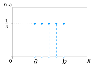
In probability theory and statistics, the discrete uniform distribution is a symmetric probability distribution wherein a finite number of values are equally likely to be observed; every one of n values has equal probability 1/n. Another way of saying "discrete uniform distribution" would be "a known, finite number of outcomes equally likely to happen".
Sample size determination or estimation is the act of choosing the number of observations or replicates to include in a statistical sample. The sample size is an important feature of any empirical study in which the goal is to make inferences about a population from a sample. In practice, the sample size used in a study is usually determined based on the cost, time, or convenience of collecting the data, and the need for it to offer sufficient statistical power. In complex studies, different sample sizes may be allocated, such as in stratified surveys or experimental designs with multiple treatment groups. In a census, data is sought for an entire population, hence the intended sample size is equal to the population. In experimental design, where a study may be divided into different treatment groups, there may be different sample sizes for each group.
In econometrics and statistics, the generalized method of moments (GMM) is a generic method for estimating parameters in statistical models. Usually it is applied in the context of semiparametric models, where the parameter of interest is finite-dimensional, whereas the full shape of the data's distribution function may not be known, and therefore maximum likelihood estimation is not applicable.
In statistics, kernel density estimation (KDE) is the application of kernel smoothing for probability density estimation, i.e., a non-parametric method to estimate the probability density function of a random variable based on kernels as weights. KDE answers a fundamental data smoothing problem where inferences about the population are made, based on a finite data sample. In some fields such as signal processing and econometrics it is also termed the Parzen–Rosenblatt window method, after Emanuel Parzen and Murray Rosenblatt, who are usually credited with independently creating it in its current form. One of the famous applications of kernel density estimation is in estimating the class-conditional marginal densities of data when using a naive Bayes classifier, which can improve its prediction accuracy.
This glossary of statistics and probability is a list of definitions of terms and concepts used in the mathematical sciences of statistics and probability, their sub-disciplines, and related fields. For additional related terms, see Glossary of mathematics and Glossary of experimental design.
In statistics, the method of moments is a method of estimation of population parameters. The same principle is used to derive higher moments like skewness and kurtosis.
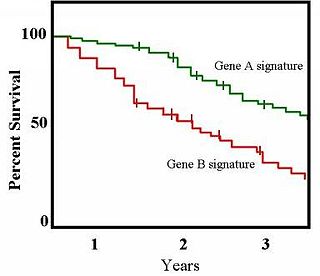
The Kaplan–Meier estimator, also known as the product limit estimator, is a non-parametric statistic used to estimate the survival function from lifetime data. In medical research, it is often used to measure the fraction of patients living for a certain amount of time after treatment. In other fields, Kaplan–Meier estimators may be used to measure the length of time people remain unemployed after a job loss, the time-to-failure of machine parts, or how long fleshy fruits remain on plants before they are removed by frugivores. The estimator is named after Edward L. Kaplan and Paul Meier, who each submitted similar manuscripts to the Journal of the American Statistical Association. The journal editor, John Tukey, convinced them to combine their work into one paper, which has been cited more than 34,000 times since its publication in 1958.
In statistics, M-estimators are a broad class of extremum estimators for which the objective function is a sample average. Both non-linear least squares and maximum likelihood estimation are special cases of M-estimators. The definition of M-estimators was motivated by robust statistics, which contributed new types of M-estimators. However, M-estimators are not inherently robust, as is clear from the fact that they include maximum likelihood estimators, which are in general not robust. The statistical procedure of evaluating an M-estimator on a data set is called M-estimation.
Bootstrapping is any test or metric that uses random sampling with replacement, and falls under the broader class of resampling methods. Bootstrapping assigns measures of accuracy to sample estimates. This technique allows estimation of the sampling distribution of almost any statistic using random sampling methods.
Good–Turing frequency estimation is a statistical technique for estimating the probability of encountering an object of a hitherto unseen species, given a set of past observations of objects from different species. In drawing balls from an urn, the 'objects' would be balls and the 'species' would be the distinct colors of the balls. After drawing red balls, black balls and green balls, we would ask what is the probability of drawing a red ball, a black ball, a green ball or one of a previously unseen color.
In statistical signal processing, the goal of spectral density estimation (SDE) or simply spectral estimation is to estimate the spectral density of a signal from a sequence of time samples of the signal. Intuitively speaking, the spectral density characterizes the frequency content of the signal. One purpose of estimating the spectral density is to detect any periodicities in the data, by observing peaks at the frequencies corresponding to these periodicities.
In the statistical theory of estimation, the German tank problem consists of estimating the maximum of a discrete uniform distribution from sampling without replacement. In simple terms, suppose there exists an unknown number of items which are sequentially numbered from 1 to N. A random sample of these items is taken and their sequence numbers observed; the problem is to estimate N from these observed numbers.
In survey methodology, the design effect is a measure of the expected impact of a sampling design on the variance of an estimator for some parameter. It is calculated as the ratio of the variance of an estimator based on a sample from an (often) complex sampling design, to the variance of an alternative estimator based on a simple random sample (SRS) of the same number of elements. The can be used to adjust the variance of an estimator in cases where the sample is not drawn using simple random sampling. It may also be useful in sample size calculations and for quantifying the representativeness of a sample. The term "design effect" was coined by Leslie Kish in 1965.
In statistics, the Horvitz–Thompson estimator, named after Daniel G. Horvitz and Donovan J. Thompson, is a method for estimating the total and mean of a pseudo-population in a stratified sample by applying inverse probability weighting to account for the difference in the sampling distribution between the collected data and the a target population. The Horvitz–Thompson estimator is frequently applied in survey analyses and can be used to account for missing data, as well as many sources of unequal selection probabilities.
Inverse probability weighting is a statistical technique for estimating quantities related to a population other than the one from which the data was collected. Study designs with a disparate sampling population and population of target inference are common in application. There may be prohibitive factors barring researchers from directly sampling from the target population such as cost, time, or ethical concerns. A solution to this problem is to use an alternate design strategy, e.g. stratified sampling. Weighting, when correctly applied, can potentially improve the efficiency and reduce the bias of unweighted estimators.
The ratio estimator is a statistical estimator for the ratio of means of two random variables. Ratio estimates are biased and corrections must be made when they are used in experimental or survey work. The ratio estimates are asymmetrical and symmetrical tests such as the t test should not be used to generate confidence intervals.
1 2 3 4 Chapman, D.G. (1951). "Some properties of the hypergeometric distribution with applications to zoological sample censuses".{{cite journal}}: Cite journal requires |journal= (help)
↑ Sadinle, Mauricio (2009-10-01). "Transformed Logit Confidence Intervals for Small Populations in Single Capture–Recapture Estimation". Communications in Statistics - Simulation and Computation. 38 (9): 1909–1924. doi:10.1080/03610910903168595. ISSN0361-0918. S2CID205556773.
↑ Drenner, Ray (1978). "Capture probability: the role of zooplankter escape in the selective feeding of planktivorous fish". Journal of the Fisheries Board of Canada. 35 (10): 1370–1373. doi:10.1139/f78-215.
↑ William J. Sutherland, ed. (1996). Ecological Census Techniques: A Handbook. Cambridge University Press. ISBN0-521-47815-4.
↑ Maunder M.N. (2003) Paradigm shifts in fisheries stock assessment: from integrated analysis to Bayesian analysis and back again. Natural Resource Modeling 16:465–475
↑ Maunder, M.N. (2001) Integrated Tagging and Catch-at-Age Analysis (ITCAAN). In Spatial Processes and Management of Fish Populations, edited by G.H. Kruse, N. Bez, A. Booth, M.W. Dorn, S. Hills, R.N. Lipcius, D. Pelletier, C. Roy, S.J. Smith, and D. Witherell, Alaska Sea Grant College Program Report No. AK-SG-01-02, University of Alaska Fairbanks, pp. 123–146.
Besbeas, P; Freeman, S. N.; Morgan, B. J. T.; Catchpole, E. A. (2002). "Integrating mark-recapture-recovery and census data to estimate animal abundance and demographic parameters". Biometrics. 58 (3): 540–547. doi:10.1111/j.0006-341X.2002.00540.x. PMID12229988. S2CID30426391.
Martin-Löf, P. (1961). "Mortality rate calculations on ringed birds with special reference to the Dunlin Calidris alpina". Arkiv för Zoologi (Zoology Files), Kungliga Svenska Vetenskapsakademien (The Royal Swedish Academy of Sciences) Serie 2. Band 13 (21).
Phillips, C. A.; M. J. Dreslik; J. R. Johnson; J. E. Petzing (2001). "Application of population estimation to pond breeding salamanders". Transactions of the Illinois Academy of Science. 94 (2): 111–118.
Royle, J. A.; R. M. Dorazio (2008). Hierarchical Modeling and Inference in Ecology. Elsevier. ISBN978-1-930665-55-2.
Seber, G.A.F. (2002). The Estimation of Animal Abundance and Related Parameters. Caldwel, New Jersey: Blackburn Press. ISBN1-930665-55-5.
Williams, B. K.; J. D. Nichols; M. J. Conroy (2002). Analysis and Management of Animal Populations. San Diego, California: Academic Press. ISBN0-12-754406-2.
Chao, A; Tsay, P. K.; Lin, S. H.; Shau, W. Y.; Chao, D. Y. (2001). "The applications of capture-recapture models to epidemiological data". Statistics in Medicine. 20 (20): 3123–3157. doi:10.1002/sim.996. PMID11590637. S2CID78437.
Further reading
Bonett, D.G.; Woodward, J.A.; Bentler, P.M. (1986). "A Linear Model for Estimating the Size of a Closed Population". British Journal of Mathematical and Statistical Psychology. 39: 28–40. doi:10.1111/j.2044-8317.1986.tb00843.x. PMID3768264.
Evans, M.A.; Bonett, D.G.; McDonald, L. (1994). "A General Theory for Analyzing Capture-recapture Data in Closed Populations". Biometrics. 50 (2): 396–405. doi:10.2307/2533383. JSTOR2533383.
Lincoln, F. C. (1930). "Calculating Waterfowl Abundance on the Basis of Banding Returns". United States Department of Agriculture Circular. 118: 1–4.
Petersen, C. G. J. (1896). "The Yearly Immigration of Young Plaice Into the Limfjord From the German Sea", Report of the Danish Biological Station (1895), 6, 5–84.
Schofield, J. R. (2007). "Beyond Defect Removal: Latent Defect Estimation With Capture-Recapture Method", Crosstalk, August 2007; 27–29.
This page is based on this Wikipedia article Text is available under the CC BY-SA 4.0 license; additional terms may apply. Images, videos and audio are available under their respective licenses.

 Collar-tagged rock hyrax
 Ring-tagged Jackdaw
 Marked Chittenango ovate amber snail
 Tagged Common Ringlet