Markov boundary
A Markov boundary of  in
in  is a subset
  of , such that itself is a Markov blanket of , but any proper subset of is not a Markov blanket of . In other words, a Markov boundary is a minimal Markov blanket.
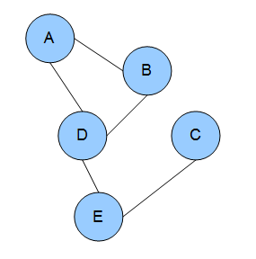
The Markov boundary of a node  in a Bayesian network is the set of nodes composed of 's parents, 's children, and 's children's other parents. In a Markov random field, the Markov boundary for a node is the set of its neighboring nodes. In a dependency network, the Markov boundary for a node is the set of its parents.
Uniqueness of Markov boundary
The Markov boundary always exists. Under some mild conditions, the Markov boundary is unique. However, for most practical and theoretical scenarios multiple Markov boundaries may provide alternative solutions. [2] When there are multiple Markov boundaries, quantities measuring causal effect could fail. [3]
A Bayesian network is a probabilistic graphical model that represents a set of variables and their conditional dependencies via a directed acyclic graph (DAG). While it is one of several forms of causal notation, causal networks are special cases of Bayesian networks. Bayesian networks are ideal for taking an event that occurred and predicting the likelihood that any one of several possible known causes was the contributing factor. For example, a Bayesian network could represent the probabilistic relationships between diseases and symptoms. Given symptoms, the network can be used to compute the probabilities of the presence of various diseases.

In probability theory and statistics, the term Markov property refers to the memoryless property of a stochastic process, which means that its future evolution is independent of its history. It is named after the Russian mathematician Andrey Markov. The term strong Markov property is similar to the Markov property, except that the meaning of "present" is defined in terms of a random variable known as a stopping time.
A graphical model or probabilistic graphical model (PGM) or structured probabilistic model is a probabilistic model for which a graph expresses the conditional dependence structure between random variables. They are commonly used in probability theory, statistics—particularly Bayesian statistics—and machine learning.
In statistics, Gibbs sampling or a Gibbs sampler is a Markov chain Monte Carlo (MCMC) algorithm for sampling from a specified multivariate probability distribution when direct sampling from the joint distribution is difficult, but sampling from the conditional distribution is more practical. This sequence can be used to approximate the joint distribution ; to approximate the marginal distribution of one of the variables, or some subset of the variables ; or to compute an integral. Typically, some of the variables correspond to observations whose values are known, and hence do not need to be sampled.
Belief propagation, also known as sum–product message passing, is a message-passing algorithm for performing inference on graphical models, such as Bayesian networks and Markov random fields. It calculates the marginal distribution for each unobserved node, conditional on any observed nodes. Belief propagation is commonly used in artificial intelligence and information theory, and has demonstrated empirical success in numerous applications, including low-density parity-check codes, turbo codes, free energy approximation, and satisfiability.

In probability theory, conditional independence describes situations wherein an observation is irrelevant or redundant when evaluating the certainty of a hypothesis. Conditional independence is usually formulated in terms of conditional probability, as a special case where the probability of the hypothesis given the uninformative observation is equal to the probability without. If is the hypothesis, and and are observations, conditional independence can be stated as an equality:
The Markov condition, sometimes called the Markov assumption, is an assumption made in Bayesian probability theory, that every node in a Bayesian network is conditionally independent of its nondescendants, given its parents. Stated loosely, it is assumed that a node has no bearing on nodes which do not descend from it. In a DAG, this local Markov condition is equivalent to the global Markov condition, which states that d-separations in the graph also correspond to conditional independence relations. This also means that a node is conditionally independent of the entire network, given its Markov blanket.
In the domain of physics and probability, a Markov random field (MRF), Markov network or undirected graphical model is a set of random variables having a Markov property described by an undirected graph. In other words, a random field is said to be a Markov random field if it satisfies Markov properties. The concept originates from the Sherrington–Kirkpatrick model.
In statistics, econometrics, epidemiology and related disciplines, the method of instrumental variables (IV) is used to estimate causal relationships when controlled experiments are not feasible or when a treatment is not successfully delivered to every unit in a randomized experiment. Intuitively, IVs are used when an explanatory variable of interest is correlated with the error term (endogenous), in which case ordinary least squares and ANOVA give biased results. A valid instrument induces changes in the explanatory variable but has no independent effect on the dependent variable and is not correlated with the error term, allowing a researcher to uncover the causal effect of the explanatory variable on the dependent variable.
In mathematics, the Gibbs measure, named after Josiah Willard Gibbs, is a probability measure frequently seen in many problems of probability theory and statistical mechanics. It is a generalization of the canonical ensemble to infinite systems. The canonical ensemble gives the probability of the system X being in state x as
In statistics, ignorability is a feature of an experiment design whereby the method of data collection does not depend on the missing data. A missing data mechanism such as a treatment assignment or survey sampling strategy is "ignorable" if the missing data matrix, which indicates which variables are observed or missing, is independent of the missing data conditional on the observed data.

In the philosophy of science, a causal model is a conceptual model that describes the causal mechanisms of a system. Several types of causal notation may be used in the development of a causal model. Causal models can improve study designs by providing clear rules for deciding which independent variables need to be included/controlled for.
In statistics, missing data, or missing values, occur when no data value is stored for the variable in an observation. Missing data are a common occurrence and can have a significant effect on the conclusions that can be drawn from the data.
In the statistical analysis of observational data, propensity score matching (PSM) is a statistical matching technique that attempts to estimate the effect of a treatment, policy, or other intervention by accounting for the covariates that predict receiving the treatment. PSM attempts to reduce the bias due to confounding variables that could be found in an estimate of the treatment effect obtained from simply comparing outcomes among units that received the treatment versus those that did not. Paul R. Rosenbaum and Donald Rubin introduced the technique in 1983.
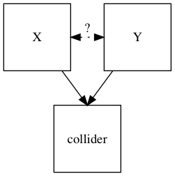
In statistics and causal graphs, a variable is a collider when it is causally influenced by two or more variables. The name "collider" reflects the fact that in graphical models, the arrow heads from variables that lead into the collider appear to "collide" on the node that is the collider. They are sometimes also referred to as inverted forks.
Exponential Random Graph Models (ERGMs) are a family of statistical models for analyzing data from social and other networks. Examples of networks examined using ERGM include knowledge networks, organizational networks, colleague networks, social media networks, networks of scientific development, and others.
A graphoid is a set of statements of the form, "X is irrelevant to Y given that we know Z" where X, Y and Z are sets of variables. The notion of "irrelevance" and "given that we know" may obtain different interpretations, including probabilistic, relational and correlational, depending on the application. These interpretations share common properties that can be captured by paths in graphs. The theory of graphoids characterizes these properties in a finite set of axioms that are common to informational irrelevance and its graphical representations.
In statistics, econometrics, epidemiology, genetics and related disciplines, causal graphs are probabilistic graphical models used to encode assumptions about the data-generating process.
Dependency networks (DNs) are graphical models, similar to Markov networks, wherein each vertex (node) corresponds to a random variable and each edge captures dependencies among variables. Unlike Bayesian networks, DNs may contain cycles. Each node is associated to a conditional probability table, which determines the realization of the random variable given its parents.
In network theory, collective classification is the simultaneous prediction of the labels for multiple objects, where each label is predicted using information about the object's observed features, the observed features and labels of its neighbors, and the unobserved labels of its neighbors. Collective classification problems are defined in terms of networks of random variables, where the network structure determines the relationship between the random variables. Inference is performed on multiple random variables simultaneously, typically by propagating information between nodes in the network to perform approximate inference. Approaches that use collective classification can make use of relational information when performing inference. Examples of collective classification include predicting attributes of individuals in a social network, classifying webpages in the World Wide Web, and inferring the research area of a paper in a scientific publication dataset.


