The mathematical principles of reinforcement (MPR) constitute of a set of mathematical equations set forth by Peter Killeen and his colleagues attempting to describe and predict the most fundamental aspects of behavior (Killeen & Sitomer, 2003).
The three key principles of MPR, arousal, constraint, and coupling, describe how incentives motivate responding, how time constrains it, and how reinforcers become associated with specific responses, respectively. Mathematical models are provided for these basic principles in order to articulate the necessary detail of actual data.
First principle: arousal
The first basic principle of MPR is arousal. Arousal refers to the activation of behavior by the presentation of incentives. An increase in activity level following repeated presentations of incentives is a fundamental aspect of conditioning. Killeen, Hanson, and Osborne (1978) proposed that adjunctive (or schedule induced) behaviors are normally occurring parts of an organism's repertoire. Delivery of incentives increases the rate of adjunctive behaviors by generating a heightened level of general activity, or arousal, in organisms.
Killeen & Hanson (1978) exposed pigeons to a single daily presentation of food in the experimental chamber and measured general activity for 15 minutes after a feeding. They showed that activity level increased slightly directly following a feeding and then decreased slowly over time. The rate of decay can be described by the following function:
The time course of the entire theoretical model of general activity is modeled by the following equation:
A = arousal
I = temporal inhibition
C = competing behaviors
To better conceptualize this model, imagine how rate of responding would appear with each of these processes individually. In the absence of temporal inhibition or competing responses, arousal level would remain high and response rate would be depicted as an almost horizontal line with a very small negative slope. Directly following food presentation, temporal inhibition is at its maximum level. It decreases quickly as time elapses, and response rate would be expected to increase up to the level of arousal in a short time. Competing behaviors such as goal tracking or hopper inspection are at a minimum directly after food presentation. These behaviors increase as the interval elapses, so the measure of general activity would slowly decrease. Subtracting these two curves results in the predicted level of general activity.
Killeen et al. (1978) then increased the frequency of feeding from daily to every fixed-time seconds. They showed that general activity level increased substantially from the level of daily presentation. Response rate asymptotes were highest for the highest rates of reinforcement. These experiments indicate that arousal level is proportional to rate of incitement, and the asymptotic level increases with repeated presentations of incentives. The increase in activity level with repeated presentation of incentives is called cumulation of arousal. The first principle of MPR states that arousal level is proportional to rate of reinforcement, , where:
A= arousal level
a= specific activation
r= rate of reinforcement
(Killeen & Sitomer, 2003).
Second principle: constraint
An obvious but often overlooked factor when analyzing response distributions is that responses are not instantaneous, but take some amount of time to emit (Killeen, 1994). These ceilings on response rate are often accounted for by competition from other responses, but less often for the fact that responses cannot always be emitted at the same rate at which they are elicited (Killeen & Sitomer, 2003). This limiting factor must be taken into account in order to correctly characterize what responding could be theoretically, and what it will be empirically.
An organism may receive impulses to respond at a certain rate. At low rates of reinforcement, the elicited rate and emitted rate will approximate each other. At high rates of reinforcement, however, this elicited rate is subdued by the amount of time it takes to emit a response. Response rate, , is typically measured as the number of responses occurring in an epoch divided by the duration of an epoch. The reciprocal of gives the typical measure of the inter response (IRT), the average time from the start of one response to the start of another (Killeen & Sitomer, 2003). This is actually the cycle time rather than the time between responses. According to Killeen & Sitomer (2003), the IRT consists of two subintervals, the time required to emit a response, plus the time between responses, . Therefore, response rate can be measured either by dividing the number of responses by the cycle time:
,
or as the number of responses divided by the actual time between responses:
.
This instantaneous rate, may be the best measure to use, as the nature of the operandum may change arbitrarily within an experiment (Killeen & Sitomer, 2003).
Killeen, Hall, Reilly, and Kettle (2002) showed that if instantaneous rate of responding is proportional to rate of reinforcement, , then a fundamental equation for MPR results. Killeen & Sitomer (2003) showed that:
if
then ,
and rearranging gives:
While responses may be elicited at a rate proportional to , they can only be emitted at rate due to constraint. The second principle of MPR states that the time required to emit a response constrains response rate (Killeen & Sitomer, 2003).
Third principle: coupling
Coupling is the final concept of MPR that ties all of the processes together and allows for specific predictions of behavior with different schedules of reinforcement. Coupling refers to the association between responses and reinforcers. The target response is the response of interest to the experimenter, but any response can become associated with a reinforcer. Contingencies of reinforcement refer to how a reinforcer is scheduled with respect to the target response (Killeen & Sitomer, 2003), and the specific schedules of reinforcement in effect determine how responses are coupled to the reinforcer. The third principle of MPR states that the degree of coupling between a response and reinforcer decreases with the distance between them (Killeen & Sitomer, 2003). Coupling coefficients, designated as , are given for the different schedules of reinforcement. When the coupling coefficients are inserted into the activation-constraint model, complete models of conditioning are derived:
This is the fundamental equation of MPR. The dot after the is a placeholder for the specific contingencies of reinforcement under study (Killeen & Sitomer, 2003).
Fixed-ratio reinforcement schedules
The rate of reinforcement for fixed-ratio schedules is easy to calculate, as reinforcement rate is directly proportional to response rate and inversely proportional to ratio requirement (Killeen, 1994). The schedule feedback function is therefore:
.
Substituting this function into the complete model gives the equation of motion for ratio schedules (Killeen & Sitomer, 2003). Killeen (1994, 2003) showed that the most recent response in a sequence of responses is weighted most heavily and given a weight of , leaving for the remaining responses. The penultimate response receives , the third back receives . The th response back is given a weight of
The sum of this series is the coupling coefficient for fixed-ratio schedules:
The continuous approximation of this is:
where is the intrinsic rate of memory decay. Inserting the reinforcement rate and coupling coefficient into the activation-constraint model gives the predicted response rates for FR schedules:
This equation predicts low response rates at low ratio requirements due to the displacement of memory by consummatory behavior. However, these low rates are not always found. Coupling of responses may extend back beyond the preceding reinforcer, and an extra parameter, is added to account for this. Killeen & Sitomer (2003) showed that the coupling coefficient for FR schedules then becomes:
is the number of responses preceding the prior reinforcer that contribute to response strength. which ranges from 0 to 1 is then the degree of erasure of the target response from memory with the delivery of a reinforcer. () If , erasure is complete and the simpler FR equation can be used.
Variable-ratio reinforcement schedules
According to Killeen & Sitomer (2003), the duration of a response can affect the rate of memory decay. When response durations vary, either within or between organisms, then a more complete model is needed, and is replaced with yielding:
Idealized variable-ratio schedules with a mean response requirement of have a constant probability of of a response ending in reinforcement (Bizo, Kettle, & Killeen, 2001). The last response ending in reinforcement must always occur and receives strengthening of . The penultimate response occurs with probability and receives a strengthening of . The sum of this process up to infinity is (Killeen 2001, Appendix):
The coupling coefficient for VR schedules ends up being:
Multiplying by degree of erasure of memory gives:
The coupling coefficient can then be inserted into the activation-constraint model just as the coupling coefficient for FR schedules to yield predicted response rates under VR schedules:
In interval schedules, the schedule feedback function is
where is the minimum average time between reinforcers (Killeen, 1994). Coupling in interval schedules is weaker than ratio schedules, as interval schedules equally strengthen all responses preceding the target rather than just the target response. Only some proportion of memory is strengthened. With a response requirement, the final, target response must receive strength of . All preceding responses, target or non-target, receive a strengthening of .
Fixed-time schedules are the simplest time dependent schedules in which organisms must simply wait t seconds for an incentive. Killeen (1994) reinterpreted temporal requirements as response requirements and integrated the contents of memory from one incentive to the next. This gives the contents of memory to be:
N
MN= lò e-lndn
0
This is the degree of saturation in memory of all responses, both target and non-target, elicited in the context (Killeen, 1994). Solving this equation gives the coupling coefficient for fixed-time schedules:
c=r(1-e-lbt)
where is the proportion of target responses in the response trajectory. Expanding into a power series gives the following approximation:
c» rlbt
1+lbt
This equation predicts serious instability for non-contingent schedules of reinforcement.
Fixed-interval schedules are guaranteed a strengthening of a target response, b=w1, as reinforcement is contingent on this final, contiguous response (Killeen, 1994). This coupling is equivalent to the coupling on FR 1 schedules
w1=b=1-e-l.
The remainder of coupling is due to the memory of preceding behavior. The coupling coefficient for FI schedules is:
c= b +r(1- b -e-lbt).
Variable-time schedules are similar to random ratio schedules in that there is a constant probability of reinforcement, but these reinforcers are set up in time rather than responses. The probability of no reinforcement occurring before some time t’ is an exponential function of that time with the time constant t being the average IRI of the schedule (Killeen, 1994). To derive the coupling coefficient, the probability of the schedule not having ended, weighted by the contents of memory, must be integrated.
∞
M= lò e-n’t/te-ln’ dn’
0
In this equation, t’=n’t, where t is a small unit of time. Killeen (1994) explains that the first exponential term is the reinforcement distribution, whereas the second term is the weighting of this distribution in memory. Solving this integral and multiplying by the coupling constant r, gives the extent to which memory is filled on VT schedules:
c=rlbt
1+lbt
This is the same coupling coefficient as an FT schedule, except it is an exact solution for VT schedules rather than an approximation. Once again, the feedback function on these non-contingent schedules predicts serious instability in responding.
As with FI schedules, variable-interval schedules are guaranteed a target response coupling of b. Simply adding b to the VT equation gives:
∞
M= b+ lò e-n’t/te-ln’ dn’
1
Solving the integral and multiplying by r gives the coupling coefficient for VI schedules:
c= b+(1-b) rlbt
1+lbt
The coupling coefficients for all of the schedules are inserted into the activation-constraint model to yield the predicted, overall response rate. The third principle of MPR states that the coupling between a response and a reinforcer decreases with increased time between them (Killeen & Sitomer, 2003).
Mathematical principles of reinforcement describe how incentives fuel behavior, how time constrains it, and how contingencies direct it. It is a general theory of reinforcement that combines both contiguity and correlation as explanatory processes of behavior. Many responses preceding reinforcement may become correlated with the reinforcer, but the final response receives the greatest weight in memory. Specific models are provided for the three basic principles to articulate predicted response patterns in many different situations and under different schedules of reinforcement. Coupling coefficients for each reinforcement schedule are derived and inserted into the fundamental equation to yield overall predicted response rates.
Related Research Articles
In a chemical reaction, chemical equilibrium is the state in which both the reactants and products are present in concentrations which have no further tendency to change with time, so that there is no observable change in the properties of the system. This state results when the forward reaction proceeds at the same rate as the reverse reaction. The reaction rates of the forward and backward reactions are generally not zero, but they are equal. Thus, there are no net changes in the concentrations of the reactants and products. Such a state is known as dynamic equilibrium.
The propagation constant of a sinusoidal electromagnetic wave is a measure of the change undergone by the amplitude and phase of the wave as it propagates in a given direction. The quantity being measured can be the voltage, the current in a circuit, or a field vector such as electric field strength or flux density. The propagation constant itself measures the change per unit length, but it is otherwise dimensionless. In the context of two-port networks and their cascades, propagation constant measures the change undergone by the source quantity as it propagates from one port to the next.
A low-pass filter is a filter that passes signals with a frequency lower than a selected cutoff frequency and attenuates signals with frequencies higher than the cutoff frequency. The exact frequency response of the filter depends on the filter design. The filter is sometimes called a high-cut filter, or treble-cut filter in audio applications. A low-pass filter is the complement of a high-pass filter.
The Grashof number (Gr) is a dimensionless number in fluid dynamics and heat transfer which approximates the ratio of the buoyancy to viscous force acting on a fluid. It frequently arises in the study of situations involving natural convection and is analogous to the Reynolds number. It's believed to be named after Franz Grashof. Though this grouping of terms had already been in use, it wasn't named until around 1921, 28 years after Franz Grashof's death. It's not very clear why the grouping was named after him.
Flight dynamics is the science of air vehicle orientation and control in three dimensions. The three critical flight dynamics parameters are the angles of rotation in three dimensions about the vehicle's center of gravity (cg), known as pitch, roll and yaw.
The laser diode rate equations model the electrical and optical performance of a laser diode. This system of ordinary differential equations relates the number or density of photons and charge carriers (electrons) in the device to the injection current and to device and material parameters such as carrier lifetime, photon lifetime, and the optical gain.
The Lotka–Volterra equations, also known as the predator–prey equations, are a pair of first-order nonlinear differential equations, frequently used to describe the dynamics of biological systems in which two species interact, one as a predator and the other as prey. The populations change through time according to the pair of equations:
A vibration in a string is a wave. Resonance causes a vibrating string to produce a sound with constant frequency, i.e. constant pitch. If the length or tension of the string is correctly adjusted, the sound produced is a musical tone. Vibrating strings are the basis of string instruments such as guitars, cellos, and pianos.
The equilibrium constant of a chemical reaction is the value of its reaction quotient at chemical equilibrium, a state approached by a dynamic chemical system after sufficient time has elapsed at which its composition has no measurable tendency towards further change. For a given set of reaction conditions, the equilibrium constant is independent of the initial analytical concentrations of the reactant and product species in the mixture. Thus, given the initial composition of a system, known equilibrium constant values can be used to determine the composition of the system at equilibrium. However, reaction parameters like temperature, solvent, and ionic strength may all influence the value of the equilibrium constant.
The Duffing equation, named after Georg Duffing (1861–1944), is a non-linear second-order differential equation used to model certain damped and driven oscillators. The equation is given by
The Newman–Penrose (NP) formalism is a set of notation developed by Ezra T. Newman and Roger Penrose for general relativity (GR). Their notation is an effort to treat general relativity in terms of spinor notation, which introduces complex forms of the usual variables used in GR. The NP formalism is itself a special case of the tetrad formalism, where the tensors of the theory are projected onto a complete vector basis at each point in spacetime. Usually this vector basis is chosen to reflect some symmetry of the spacetime, leading to simplified expressions for physical observables. In the case of the NP formalism, the vector basis chosen is a null tetrad: a set of four null vectors—two real, and a complex-conjugate pair. The two real members asymptotically point radially inward and radially outward, and the formalism is well adapted to treatment of the propagation of radiation in curved spacetime. The Weyl scalars, derived from the Weyl tensor, are often used. In particular, it can be shown that one of these scalars— in the appropriate frame—encodes the outgoing gravitational radiation of an asymptotically flat system.
Lateral earth pressure is the pressure that soil exerts in the horizontal direction. The lateral earth pressure is important because it affects the consolidation behavior and strength of the soil and because it is considered in the design of geotechnical engineering structures such as retaining walls, basements, tunnels, deep foundations and braced excavations.
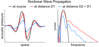
Nonlinear acoustics (NLA) is a branch of physics and acoustics dealing with sound waves of sufficiently large amplitudes. Large amplitudes require using full systems of governing equations of fluid dynamics and elasticity. These equations are generally nonlinear, and their traditional linearization is no longer possible. The solutions of these equations show that, due to the effects of nonlinearity, sound waves are being distorted as they travel.
Racah's W-coefficients were introduced by Giulio Racah in 1942. These coefficients have a purely mathematical definition. In physics they are used in calculations involving the quantum mechanical description of angular momentum, for example in atomic theory.
The Liénard–Wiechert potentials describe the classical electromagnetic effect of a moving electric point charge in terms of a vector potential and a scalar potential in the Lorenz gauge. Stemming directly from Maxwell's equations, these describe the complete, relativistically correct, time-varying electromagnetic field for a point charge in arbitrary motion, but are not corrected for quantum mechanical effects. Electromagnetic radiation in the form of waves can be obtained from these potentials. These expressions were developed in part by Alfred-Marie Liénard in 1898 and independently by Emil Wiechert in 1900.
In electrochemistry, the Butler–Volmer equation, also known as Erdey-Grúz–Volmer equation, is one of the most fundamental relationships in electrochemical kinetics. It describes how the electrical current through an electrode depends on the voltage difference between the electrode and the bulk electrolyte for a simple, unimolecular redox reaction, considering that both a cathodic and an anodic reaction occur on the same electrode:
Thermo-mechanical fatigue is the overlay of a cyclical mechanical loading, that leads to fatigue of a material, with a cyclical thermal loading. Thermo-mechanical fatigue is an important point that needs to be considered, when constructing turbine engines or gas turbines.
In theoretical physics, the dual graviton is a hypothetical elementary particle that is a dual of the graviton under electric-magnetic duality, as an S-duality, predicted by some formulations of supergravity in eleven dimensions.
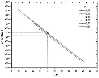
The alpha-beta model is a mathematical equation used to describe the velocity of fatigue crack growth, da / dN, as a function of a constant amplitude load driving force ΔK where its constants α and β are obtained through a semi-empirical process. Originally the alpha-beta model was developed and tested from data generated in tests using commercial grade Titanium and Aluminium Alloy 2524-T3 both the structural materials of great interest aeronautical. This model is applied in two situations: the individual that conforms to the experimental data of a single test and can be compared to Paris' law; and the generalized one that tries to represent in a bi-parametric way the effects of R - ratio between the tensions intensity, minimum and maximum - for a set of tests in the same material.
A crack growth equation is used for calculating the size of a fatigue crack growing from cyclic loads. The growth of fatigue cracks can result in catastrophic failure, particularly in the case of aircraft. A crack growth equation can be used to ensure safety, both in the design phase and during operation, by predicting the size of cracks. In critical structure, loads can be recorded and used to predict the size of cracks to ensure maintenance or retirement occurs prior to any of the cracks failing.
References
Sources
Bizo, L. A., Kettle, L. C. & Killeen, P. R. (2001). "Animals don't always respond faster for more food: The paradoxical incentive effect." Animal Learning & Behavior, 29, 66-78.
Killeen, P.R. (1994). "Mathematical principles of reinforcement." Behavioral and Brain Sciences, 17, 105-172.
Killeen, P. R., Hall, S. S., Reilly, M. P., & Kettle, L. C. (2002). "Molecular analyses of the principal components of response strength." Journal of the Experimental Analysis of Behavior, 78, 127-160.
Killeen, P. R., Hanson, S. J., & Osborne, S. R. (1978). "Arousal: Its genesis and manifestation as response rate." Psychological review. Vol 85 No 6. p.571-81
Killeen, P. R. & Sitomer, M. T. (2003). "MPR." Behavioural Processes, 62, 49-64
This page is based on this Wikipedia article Text is available under the CC BY-SA 4.0 license; additional terms may apply. Images, videos and audio are available under their respective licenses.