Illustration via an example
Suppose a certain random variable takes values in the set of non-negative integers 1, 2, 3, . . . . A simple random sample of size 20 is taken, yielding the following data set. It is desired to test the null hypothesis that the population from which this sample was taken follows a Poisson distribution.

The maximum likelihood estimate of the population average is 3.3. One could apply Pearson's chi-square test of whether the population distribution is a Poisson distribution with expected value 3.3. However, the null hypothesis did not specify that it was that particular Poisson distribution, but only that it is some Poisson distribution, and the number 3.3 came from the data, not from the null hypothesis. A rule of thumb says that when a parameter is estimated, one reduces the number of degrees of freedom by 1, in this case from 9 (since there are 10 cells) to 8. One might hope that the resulting test statistic would have approximately a chi-square distribution when the null hypothesis is true. However, that is not in general the case when maximum-likelihood estimation is used. It is however true asymptotically when minimum chi-square estimation is used.
Finding the minimum chi-square estimate
The minimum chi-square estimate of the population mean λ is the number that minimizes the chi-square statistic

where a is the estimated expected number in the "> 8" cell, and "20" appears because it is the sample size. The value of a is 20 times the probability that a Poisson-distributed random variable exceeds 8, and it is easily calculated as 1 minus the sum of the probabilities corresponding to 0 through 8. By trivial algebra, the last term reduces simply to a. Numerical computation shows that the value of λ that minimizes the chi-square statistic is about 3.5242. That is the minimum chi-square estimate of λ. For that value of λ, the chi-square statistic is about 3.062764. There are 10 cells. If the null hypothesis had specified a single distribution, rather than requiring λ to be estimated, then the null distribution of the test statistic would be a chi-square distribution with 10 − 1 = 9 degrees of freedom. Since λ had to be estimated, one additional degree of freedom is lost. The expected value of a chi-square random variable with 8 degrees of freedom is 8. Thus the observed value, 3.062764, is quite modest, and the null hypothesis is not rejected.
In statistics, the likelihood-ratio test assesses the goodness of fit of two competing statistical models based on the ratio of their likelihoods, specifically one found by maximization over the entire parameter space and another found after imposing some constraint. If the constraint is supported by the observed data, the two likelihoods should not differ by more than sampling error. Thus the likelihood-ratio test tests whether this ratio is significantly different from one, or equivalently whether its natural logarithm is significantly different from zero.

In probability theory and statistics, the exponential distribution or negative exponential distribution is the probability distribution of the time between events in a Poisson point process, i.e., a process in which events occur continuously and independently at a constant average rate. It is a particular case of the gamma distribution. It is the continuous analogue of the geometric distribution, and it has the key property of being memoryless. In addition to being used for the analysis of Poisson point processes it is found in various other contexts.

In probability theory and statistics, the chi-squared distribution with degrees of freedom is the distribution of a sum of the squares of independent standard normal random variables. The chi-squared distribution is a special case of the gamma distribution and is one of the most widely used probability distributions in inferential statistics, notably in hypothesis testing and in construction of confidence intervals. This distribution is sometimes called the central chi-squared distribution, a special case of the more general noncentral chi-squared distribution.

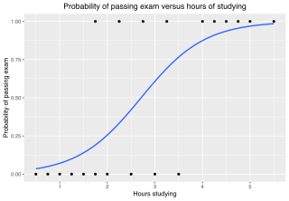
In statistics, the logistic model is a statistical model that models the probability of an event taking place by having the log-odds for the event be a linear combination of one or more independent variables. In regression analysis, logistic regression is estimating the parameters of a logistic model. Formally, in binary logistic regression there is a single binary dependent variable, coded by an indicator variable, where the two values are labeled "0" and "1", while the independent variables can each be a binary variable or a continuous variable. The corresponding probability of the value labeled "1" can vary between 0 and 1, hence the labeling; the function that converts log-odds to probability is the logistic function, hence the name. The unit of measurement for the log-odds scale is called a logit, from logistic unit, hence the alternative names. See § Background and § Definition for formal mathematics, and § Example for a worked example.
Pearson's chi-squared test is a statistical test applied to sets of categorical data to evaluate how likely it is that any observed difference between the sets arose by chance. It is the most widely used of many chi-squared tests – statistical procedures whose results are evaluated by reference to the chi-squared distribution. Its properties were first investigated by Karl Pearson in 1900. In contexts where it is important to improve a distinction between the test statistic and its distribution, names similar to Pearson χ-squared test or statistic are used.

A chi-squared test is a statistical hypothesis test used in the analysis of contingency tables when the sample sizes are large. In simpler terms, this test is primarily used to examine whether two categorical variables are independent in influencing the test statistic. The test is valid when the test statistic is chi-squared distributed under the null hypothesis, specifically Pearson's chi-squared test and variants thereof. Pearson's chi-squared test is used to determine whether there is a statistically significant difference between the expected frequencies and the observed frequencies in one or more categories of a contingency table. For contingency tables with smaller sample sizes, a Fisher's exact test is used instead.
In statistics, G-tests are likelihood-ratio or maximum likelihood statistical significance tests that are increasingly being used in situations where chi-squared tests were previously recommended.
In probability theory and statistics, the noncentral F-distribution is a continuous probability distribution that is a noncentral generalization of the (ordinary) F-distribution. It describes the distribution of the quotient (X/n1)/(Y/n2), where the numerator X has a noncentral chi-squared distribution with n1 degrees of freedom and the denominator Y has a central chi-squared distribution with n2 degrees of freedom. It is also required that X and Y are statistically independent of each other.
In statistics, the score test assesses constraints on statistical parameters based on the gradient of the likelihood function—known as the score—evaluated at the hypothesized parameter value under the null hypothesis. Intuitively, if the restricted estimator is near the maximum of the likelihood function, the score should not differ from zero by more than sampling error. While the finite sample distributions of score tests are generally unknown, they have an asymptotic χ2-distribution under the null hypothesis as first proved by C. R. Rao in 1948, a fact that can be used to determine statistical significance.
In statistics, the Vuong closeness test is a likelihood-ratio-based test for model selection using the Kullback–Leibler information criterion. This statistic makes probabilistic statements about two models. They can be nested, strictly non-nested or partially non-nested. The statistic tests the null hypothesis that the two models are equally close to the true data generating process, against the alternative that one model is closer. It cannot make any decision whether the "closer" model is the true model.
The goodness of fit of a statistical model describes how well it fits a set of observations. Measures of goodness of fit typically summarize the discrepancy between observed values and the values expected under the model in question. Such measures can be used in statistical hypothesis testing, e.g. to test for normality of residuals, to test whether two samples are drawn from identical distributions, or whether outcome frequencies follow a specified distribution. In the analysis of variance, one of the components into which the variance is partitioned may be a lack-of-fit sum of squares.
In statistics, an exact (significance) test is a test such that if the null hypothesis is true, then all assumptions made during the derivation of the distribution of the test statistic are met. Using an exact test provides a significance test that maintains the type I error rate of the test at the desired significance level of the test. For example, an exact test at a significance level of , when repeated over many samples where the null hypothesis is true, will reject at most of the time. This is in contrast to an approximate test in which the desired type I error rate is only approximately maintained, while this approximation may be made as close to as desired by making the sample size sufficiently large.

In probability theory and statistics, the noncentral chi-squared distribution is a noncentral generalization of the chi-squared distribution. It often arises in the power analysis of statistical tests in which the null distribution is a chi-squared distribution; important examples of such tests are the likelihood-ratio tests.
Omnibus tests are a kind of statistical test. They test whether the explained variance in a set of data is significantly greater than the unexplained variance, overall. One example is the F-test in the analysis of variance. There can be legitimate significant effects within a model even if the omnibus test is not significant. For instance, in a model with two independent variables, if only one variable exerts a significant effect on the dependent variable and the other does not, then the omnibus test may be non-significant. This fact does not affect the conclusions that may be drawn from the one significant variable. In order to test effects within an omnibus test, researchers often use contrasts.

In probability theory and statistics, the Conway–Maxwell–Poisson distribution is a discrete probability distribution named after Richard W. Conway, William L. Maxwell, and Siméon Denis Poisson that generalizes the Poisson distribution by adding a parameter to model overdispersion and underdispersion. It is a member of the exponential family, has the Poisson distribution and geometric distribution as special cases and the Bernoulli distribution as a limiting case.
In statistics, the multinomial test is the test of the null hypothesis that the parameters of a multinomial distribution equal specified values; it is used for categorical data.

In statistics, maximum spacing estimation (MSE or MSP), or maximum product of spacing estimation (MPS), is a method for estimating the parameters of a univariate statistical model. The method requires maximization of the geometric mean of spacings in the data, which are the differences between the values of the cumulative distribution function at neighbouring data points.

In probability theory and statistics, the Poisson distribution is a discrete probability distribution that expresses the probability of a given number of events occurring in a fixed interval of time or space if these events occur with a known constant mean rate and independently of the time since the last event. It is named after French mathematician Siméon Denis Poisson. The Poisson distribution can also be used for the number of events in other specified interval types such as distance, area, or volume.
In statistics Wilks' theorem offers an asymptotic distribution of the log-likelihood ratio statistic, which can be used to produce confidence intervals for maximum-likelihood estimates or as a test statistic for performing the likelihood-ratio test.
Log-linear analysis is a technique used in statistics to examine the relationship between more than two categorical variables. The technique is used for both hypothesis testing and model building. In both these uses, models are tested to find the most parsimonious model that best accounts for the variance in the observed frequencies.


