In probability theory and statistics, the binomial distribution with parameters n and p is the discrete probability distribution of the number of successes in a sequence of n independent experiments, each asking a yes–no question, and each with its own Boolean-valued outcome: success or failure. A single success/failure experiment is also called a Bernoulli trial or Bernoulli experiment, and a sequence of outcomes is called a Bernoulli process; for a single trial, i.e., n = 1, the binomial distribution is a Bernoulli distribution. The binomial distribution is the basis for the popular binomial test of statistical significance.

In probability theory and statistics, the cumulative distribution function (CDF) of a real-valued random variable , or just distribution function of , evaluated at , is the probability that will take a value less than or equal to .

A random variable is a mathematical formalization of a quantity or object which depends on random events. The term 'random variable' in its mathematical definition refers to neither randomness nor variability but instead is a mathematical function in which
Independence is a fundamental notion in probability theory, as in statistics and the theory of stochastic processes. Two events are independent, statistically independent, or stochastically independent if, informally speaking, the occurrence of one does not affect the probability of occurrence of the other or, equivalently, does not affect the odds. Similarly, two random variables are independent if the realization of one does not affect the probability distribution of the other.

In probability theory and statistics, variance is the expected value of the squared deviation from the mean of a random variable. The standard deviation (SD) is obtained as the square root of the variance. Variance is a measure of dispersion, meaning it is a measure of how far a set of numbers is spread out from their average value. It is the second central moment of a distribution, and the covariance of the random variable with itself, and it is often represented by , , , , or .
In probability theory, the central limit theorem (CLT) states that, under appropriate conditions, the distribution of a normalized version of the sample mean converges to a standard normal distribution. This holds even if the original variables themselves are not normally distributed. There are several versions of the CLT, each applying in the context of different conditions.

In probability theory and statistics, the multivariate normal distribution, multivariate Gaussian distribution, or joint normal distribution is a generalization of the one-dimensional (univariate) normal distribution to higher dimensions. One definition is that a random vector is said to be k-variate normally distributed if every linear combination of its k components has a univariate normal distribution. Its importance derives mainly from the multivariate central limit theorem. The multivariate normal distribution is often used to describe, at least approximately, any set of (possibly) correlated real-valued random variables, each of which clusters around a mean value.
In probability theory, the law of large numbers (LLN) is a mathematical theorem that states that the average of the results obtained from a large number of independent and identical random samples converges to the true value, if it exists. More formally, the LLN states that given a sample of independent and identically distributed values, the sample mean converges to the true mean.

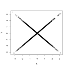
In statistics, correlation or dependence is any statistical relationship, whether causal or not, between two random variables or bivariate data. Although in the broadest sense, "correlation" may indicate any type of association, in statistics it usually refers to the degree to which a pair of variables are linearly related. Familiar examples of dependent phenomena include the correlation between the height of parents and their offspring, and the correlation between the price of a good and the quantity the consumers are willing to purchase, as it is depicted in the so-called demand curve.
In probability theory and statistics, two real-valued random variables, , , are said to be uncorrelated if their covariance, , is zero. If two variables are uncorrelated, there is no linear relationship between them.

In probability theory and statistics, the Bernoulli distribution, named after Swiss mathematician Jacob Bernoulli, is the discrete probability distribution of a random variable which takes the value 1 with probability and the value 0 with probability . Less formally, it can be thought of as a model for the set of possible outcomes of any single experiment that asks a yes–no question. Such questions lead to outcomes that are Boolean-valued: a single bit whose value is success/yes/true/one with probability p and failure/no/false/zero with probability q. It can be used to represent a coin toss where 1 and 0 would represent "heads" and "tails", respectively, and p would be the probability of the coin landing on heads. In particular, unfair coins would have

In statistics, the Pearson correlation coefficient (PCC) is a correlation coefficient that measures linear correlation between two sets of data. It is the ratio between the covariance of two variables and the product of their standard deviations; thus, it is essentially a normalized measurement of the covariance, such that the result always has a value between −1 and 1. As with covariance itself, the measure can only reflect a linear correlation of variables, and ignores many other types of relationships or correlations. As a simple example, one would expect the age and height of a sample of teenagers from a high school to have a Pearson correlation coefficient significantly greater than 0, but less than 1.

In probability theory and statistics, the Rayleigh distribution is a continuous probability distribution for nonnegative-valued random variables. Up to rescaling, it coincides with the chi distribution with two degrees of freedom. The distribution is named after Lord Rayleigh.
In probability theory and statistics, the Rademacher distribution is a discrete probability distribution where a random variate X has a 50% chance of being +1 and a 50% chance of being -1.
A ratio distribution is a probability distribution constructed as the distribution of the ratio of random variables having two other known distributions. Given two random variables X and Y, the distribution of the random variable Z that is formed as the ratio Z = X/Y is a ratio distribution.

In probability theory and statistics, the Poisson distribution is a discrete probability distribution that expresses the probability of a given number of events occurring in a fixed interval of time if these events occur with a known constant mean rate and independently of the time since the last event. It can also be used for the number of events in other types of intervals than time, and in dimension greater than 1.
A product distribution is a probability distribution constructed as the distribution of the product of random variables having two other known distributions. Given two statistically independent random variables X and Y, the distribution of the random variable Z that is formed as the product is a product distribution.
In probability theory, concentration inequalities provide mathematical bounds on the probability of a random variable deviating from some value.
In probability theory and statistics, cokurtosis is a measure of how much two random variables change together. Cokurtosis is the fourth standardized cross central moment. If two random variables exhibit a high level of cokurtosis they will tend to undergo extreme positive and negative deviations at the same time.
In probability theory and statistics, complex random variables are a generalization of real-valued random variables to complex numbers, i.e. the possible values a complex random variable may take are complex numbers. Complex random variables can always be considered as pairs of real random variables: their real and imaginary parts. Therefore, the distribution of one complex random variable may be interpreted as the joint distribution of two real random variables.