Neural cryptography

Last updated August 22, 2024

Neural cryptography is a branch of cryptography dedicated to analyzing the application of stochastic algorithms, especially artificial neural network algorithms, for use in encryption and cryptanalysis.

Definition

Artificial neural networks are well known for their ability to selectively explore the solution space of a given problem. This feature finds a natural niche of application in the field of cryptanalysis. At the same time, neural networks offer a new approach to attack ciphering algorithms based on the principle that any function could be reproduced by a neural network, which is a powerful proven computational tool that can be used to find the inverse-function of any cryptographic algorithm.

The ideas of mutual learning, self learning, and stochastic behavior of neural networks and similar algorithms can be used for different aspects of cryptography, like public-key cryptography, solving the key distribution problem using neural network mutual synchronization, hashing or generation of pseudo-random numbers.

Another idea is the ability of a neural network to separate space in non-linear pieces using "bias". It gives different probabilities of activating the neural network or not. This is very useful in the case of Cryptanalysis.

Two names are used to design the same domain of research: Neuro-Cryptography and Neural Cryptography.

The first work that it is known on this topic can be traced back to 1995 in an IT Master Thesis.

Applications

In 1995, Sebastien Dourlens applied neural networks to cryptanalyze DES by allowing the networks to learn how to invert the S-tables of the DES. The bias in DES studied through Differential Cryptanalysis by Adi Shamir is highlighted. The experiment shows about 50% of the key bits can be found, allowing the complete key to be found in a short time. Hardware application with multi micro-controllers have been proposed due to the easy implementation of multilayer neural networks in hardware.

One example of a public-key protocol is given by Khalil Shihab. He describes the decryption scheme and the public key creation that are based on a backpropagation neural network. The encryption scheme and the private key creation process are based on Boolean algebra. This technique has the advantage of small time and memory complexities. A disadvantage is the property of backpropagation algorithms: because of huge training sets, the learning phase of a neural network is very long. Therefore, the use of this protocol is only theoretical so far.

Neural key exchange protocol

The most used protocol for key exchange between two parties A and B in the practice is Diffie–Hellman key exchange protocol. Neural key exchange, which is based on the synchronization of two tree parity machines, should be a secure replacement for this method. Synchronizing these two machines is similar to synchronizing two chaotic oscillators in chaos communications.

Tree parity machine

The tree parity machine is a special type of multi-layer feedforward neural network.

It consists of one output neuron, K hidden neurons and K×N input neurons. Inputs to the network take three values:

x_{ij}\in \left\{-1,0,+1\right\}

The weights between input and hidden neurons take the values:

w_{ij}\in \left\{-L,...,0,...,+L\right\}

Output value of each hidden neuron is calculated as a sum of all multiplications of input neurons and these weights:

\sigma _{i}=\operatorname {sgn}(\sum _{j=1}^{N}w_{ij}x_{ij})

Signum is a simple function, which returns −1,0 or 1:

\operatorname {sgn}(x)={\begin{cases}-1&{\text{if }}x<0,\\0&{\text{if }}x=0,\\1&{\text{if }}x>0.\end{cases}}

If the scalar product is 0, the output of the hidden neuron is mapped to −1 in order to ensure a binary output value. The output of neural network is then computed as the multiplication of all values produced by hidden elements:

\tau =\prod _{i=1}^{K}\sigma _{i}

Output of the tree parity machine is binary.

Protocol

Each party (A and B) uses its own tree parity machine. Synchronization of the tree parity machines is achieved in these steps

Initialize random weight values
Execute these steps until the full synchronization is achieved
1. Generate random input vector X
2. Compute the values of the hidden neurons
3. Compute the value of the output neuron
4. Compare the values of both tree parity machines
  1. Outputs are the same: one of the suitable learning rules is applied to the weights
  2. Outputs are different: go to 2.1

After the full synchronization is achieved (the weights w_ij of both tree parity machines are same), A and B can use their weights as keys.
This method is known as a bidirectional learning.
One of the following learning rules^[1] can be used for the synchronization:

Hebbian learning rule:

w_{i}^{+}=g(w_{i}+\sigma _{i}x_{i}\Theta (\sigma _{i}\tau )\Theta (\tau ^{A}\tau ^{B}))

Anti-Hebbian learning rule:

w_{i}^{+}=g(w_{i}-\sigma _{i}x_{i}\Theta (\sigma _{i}\tau )\Theta (\tau ^{A}\tau ^{B}))

Random walk:

w_{i}^{+}=g(w_{i}+x_{i}\Theta (\sigma _{i}\tau )\Theta (\tau ^{A}\tau ^{B}))

Where:

\Theta (a,b)=0

if

a\neq b

otherwise

\Theta (a,b)=1

And:

g(x)

is a function that keeps the

w_{i}

in the range

\{-L,-L+1,...,0,...,L-1,L\}

Attacks and security of this protocol

In every attack it is considered, that the attacker E can eavesdrop messages between the parties A and B, but does not have an opportunity to change them.

Brute force

To provide a brute force attack, an attacker has to test all possible keys (all possible values of weights wij). By K hidden neurons, K×N input neurons and boundary of weights L, this gives (2L+1)^KN possibilities. For example, the configuration K = 3, L = 3 and N = 100 gives us 3*10²⁵³ key possibilities, making the attack impossible with today's computer power.

Learning with own tree parity machine

One of the basic attacks can be provided by an attacker, who owns the same tree parity machine as the parties A and B. He wants to synchronize his tree parity machine with these two parties. In each step there are three situations possible:

Output(A) ≠ Output(B): None of the parties updates its weights.
Output(A) = Output(B) = Output(E): All the three parties update weights in their tree parity machines.
Output(A) = Output(B) ≠ Output(E): Parties A and B update their tree parity machines, but the attacker can not do that. Because of this situation his learning is slower than the synchronization of parties A and B.

It has been proven, that the synchronization of two parties is faster than learning of an attacker. It can be improved by increasing of the synaptic depth L of the neural network. That gives this protocol enough security and an attacker can find out the key only with small probability.

Other attacks

For conventional cryptographic systems, we can improve the security of the protocol by increasing of the key length. In the case of neural cryptography, we improve it by increasing of the synaptic depth L of the neural networks. Changing this parameter increases the cost of a successful attack exponentially, while the effort for the users grows polynomially. Therefore, breaking the security of neural key exchange belongs to the complexity class NP.

Alexander Klimov, Anton Mityaguine, and Adi Shamir say that the original neural synchronization scheme can be broken by at least three different attacks—geometric, probabilistic analysis, and using genetic algorithms. Even though this particular implementation is insecure, the ideas behind chaotic synchronization could potentially lead to a secure implementation.^[2]

Permutation parity machine

The permutation parity machine is a binary variant of the tree parity machine.^[3]

It consists of one input layer, one hidden layer and one output layer. The number of neurons in the output layer depends on the number of hidden units K. Each hidden neuron has N binary input neurons:

x_{ij}\in \left\{0,1\right\}

The weights between input and hidden neurons are also binary:

w_{ij}\in \left\{0,1\right\}

Output value of each hidden neuron is calculated as a sum of all exclusive disjunctions (exclusive or) of input neurons and these weights:

\sigma _{i}=\theta _{N}(\sum _{j=1}^{N}w_{ij}\oplus x_{ij})

(⊕ means XOR).

The function $\theta _{N}(x)$ is a threshold function, which returns 0 or 1:

\theta _{N}(x)={\begin{cases}0&{\text{if }}x\leq N/2,\\1&{\text{if }}x>N/2.\end{cases}}

The output of neural network with two or more hidden neurons can be computed as the exclusive or of the values produced by hidden elements:

\tau =\bigoplus _{i=1}^{K}\sigma _{i}

Other configurations of the output layer for K>2 are also possible.^[3]

This machine has proven to be robust enough against some attacks^[4] so it could be used as a cryptographic mean, but it has been shown to be vulnerable to a probabilistic attack.^[5]

Security against quantum computers

A quantum computer is a device that uses quantum mechanisms for computation. In this device the data are stored as qubits (quantum binary digits). That gives a quantum computer in comparison with a conventional computer the opportunity to solve complicated problems in a short time, e.g. discrete logarithm problem or factorization. Algorithms that are not based on any of these number theory problems are being searched because of this property.

Neural key exchange protocol is not based on any number theory. It is based on the difference between unidirectional and bidirectional synchronization of neural networks. Therefore, something like the neural key exchange protocol could give rise to potentially faster key exchange schemes.^[2]

Related Research Articles

Linear elasticity is a mathematical model of how solid objects deform and become internally stressed by prescribed loading conditions. It is a simplification of the more general nonlinear theory of elasticity and a branch of continuum mechanics.

In statistics, an expectation–maximization (EM) algorithm is an iterative method to find (local) maximum likelihood or maximum a posteriori (MAP) estimates of parameters in statistical models, where the model depends on unobserved latent variables. The EM iteration alternates between performing an expectation (E) step, which creates a function for the expectation of the log-likelihood evaluated using the current estimate for the parameters, and a maximization (M) step, which computes parameters maximizing the expected log-likelihood found on the E step. These parameter-estimates are then used to determine the distribution of the latent variables in the next E step. It can be used, for example, to estimate a mixture of gaussians, or to solve the multiple linear regression problem.

A Hopfield network is a spin glass system used to model neural networks, based on Ernst Ising's work with Wilhelm Lenz on the Ising model of magnetic materials. Hopfield networks were first described with respect to recurrent neural networks independently by Kaoru Nakano in 1971 and Shun'ichi Amari in 1972, and with respect to biological neural networks by William Little in 1974, and were popularised by John Hopfield in 1982. Hopfield networks serve as content-addressable ("associative") memory systems with binary threshold nodes, or with continuous variables. Hopfield networks also provide a model for understanding human memory.

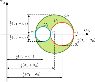
Mohr's circle is a two-dimensional graphical representation of the transformation law for the Cauchy stress tensor.

Recurrent neural networks (RNNs) are a class of artificial neural networks for sequential data processing. Unlike feedforward neural networks, which process data in a single pass, RNNs process data across multiple time steps, making them well-adapted for modelling and processing text, speech, and time series.

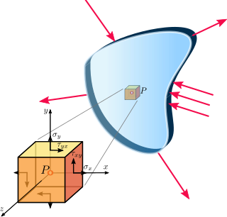
In continuum mechanics, a material is said to be under plane stress if the stress vector is zero across a particular plane. When that situation occurs over an entire element of a structure, as is often the case for thin plates, the stress analysis is considerably simplified, as the stress state can be represented by a tensor of dimension 2. A related notion, plane strain, is often applicable to very thick members.

ADALINE is an early single-layer artificial neural network and the name of the physical device that implemented this network. It was developed by professor Bernard Widrow and his doctoral student Ted Hoff at Stanford University in 1960. It is based on the perceptron. It consists of a weight, a bias and a summation function. The weights and biases were implemented by rheostats, and later, memistors.

<span class="mw-page-title-main">Biological neuron model</span> Mathematical descriptions of the properties of certain cells in the nervous system

Biological neuron models, also known as spiking neuron models, are mathematical descriptions of the conduction of electrical signals in neurons. Neurons are electrically excitable cells within the nervous system, able to fire electric signals, called action potentials, across a neural network. These mathematical models describe the role of the biophysical and geometrical characteristics of neurons on the conduction of electrical activity.

Location estimation in wireless sensor networks is the problem of estimating the location of an object from a set of noisy measurements. These measurements are acquired in a distributed manner by a set of sensors.

In the mathematical theory of artificial neural networks, universal approximation theorems are theorems of the following form: Given a family of neural networks, for each function $from a certain function space, there exists a sequence of neural networks from the family, such that according to some criterion. That is, the family of neural networks is dense in the function space.$

In mathematics, an elliptic hypergeometric series is a series Σc_n such that the ratio c_n/c_n−1 is an elliptic function of n, analogous to generalized hypergeometric series where the ratio is a rational function of n, and basic hypergeometric series where the ratio is a periodic function of the complex number n. They were introduced by Date-Jimbo-Kuniba-Miwa-Okado (1987) and Frenkel & Turaev (1997) in their study of elliptic 6-j symbols.

An affine term structure model is a financial model that relates zero-coupon bond prices to a spot rate model. It is particularly useful for deriving the yield curve – the process of determining spot rate model inputs from observable bond market data. The affine class of term structure models implies the convenient form that log bond prices are linear functions of the spot rate.

Biological motion perception is the act of perceiving the fluid unique motion of a biological agent. The phenomenon was first documented by Swedish perceptual psychologist, Gunnar Johansson, in 1973. There are many brain areas involved in this process, some similar to those used to perceive faces. While humans complete this process with ease, from a computational neuroscience perspective there is still much to be learned as to how this complex perceptual problem is solved. One tool which many research studies in this area use is a display stimuli called a point light walker. Point light walkers are coordinated moving dots that simulate biological motion in which each dot represents specific joints of a human performing an action.

In machine learning, the vanishing gradient problem is encountered when training neural networks with gradient-based learning methods and backpropagation. In such methods, during each iteration of training each of the neural networks weights receives an update proportional to the partial derivative of the error function with respect to the current weight. The problem is that as the sequence length increases, the gradient magnitude typically is expected to decrease, slowing the training process. In the worst case, this may completely stop the neural network from further training. As one example of the problem cause, traditional activation functions such as the hyperbolic tangent function have gradients in the range $[-1,1]$ , and backpropagation computes gradients by the chain rule. This has the effect of multiplying $n$ of these small numbers to compute gradients of the early layers in an $n$ -layer network, meaning that the gradient decreases exponentially with $n$ while the early layers train very slowly.

An artificial neural network (ANN) combines biological principles with advanced statistics to solve problems in domains such as pattern recognition and game-play. ANNs adopt the basic model of neuron analogues connected to each other in a variety of ways.

In the study of artificial neural networks (ANNs), the neural tangent kernel (NTK) is a kernel that describes the evolution of deep artificial neural networks during their training by gradient descent. It allows ANNs to be studied using theoretical tools from kernel methods.

A Neural Network Gaussian Process (NNGP) is a Gaussian process (GP) obtained as the limit of a certain type of sequence of neural networks. Specifically, a wide variety of network architectures converges to a GP in the infinitely wide limit, in the sense of distribution. The concept constitutes an intensional definition, i.e., a NNGP is just a GP, but distinguished by how it is obtained.

Nonlinear mixed-effects models constitute a class of statistical models generalizing linear mixed-effects models. Like linear mixed-effects models, they are particularly useful in settings where there are multiple measurements within the same statistical units or when there are dependencies between measurements on related statistical units. Nonlinear mixed-effects models are applied in many fields including medicine, public health, pharmacology, and ecology.

The spike response model (SRM) is a spiking neuron model in which spikes are generated by either a deterministic or a stochastic threshold process. In the SRM, the membrane voltage $V$ is described as a linear sum of the postsynaptic potentials (PSPs) caused by spike arrivals to which the effects of refractoriness and adaptation are added. The threshold is either fixed or dynamic. In the latter case it increases after each spike. The SRM is flexible enough to account for a variety of neuronal firing pattern in response to step current input. The SRM has also been used in the theory of computation to quantify the capacity of spiking neural networks; and in the neurosciences to predict the subthreshold voltage and the firing times of cortical neurons during stimulation with a time-dependent current stimulation. The name Spike Response Model points to the property that the two important filters $and of the model can be interpreted as the response of the membrane potential to an incoming spike (response kernel , the PSP) and to an outgoing spike (response kernel , also called refractory kernel). The SRM has been formulated in continuous time and in discrete time. The SRM can be viewed as a generalized linear model (GLM) or as an (integrated version of) a generalized integrate-and-fire model with adaptation.$

Deep backward stochastic differential equation method is a numerical method that combines deep learning with Backward stochastic differential equation (BSDE). This method is particularly useful for solving high-dimensional problems in financial derivatives pricing and risk management. By leveraging the powerful function approximation capabilities of deep neural networks, deep BSDE addresses the computational challenges faced by traditional numerical methods in high-dimensional settings.

References

↑ Singh, Ajit; Nandal, Aarti (May 2013). "Neural Cryptography for Secret Key Exchange and Encryption with AES" (PDF). International Journal of Advanced Research in Computer Science and Software Engineering. 3 (5): 376–381. ISSN 2277-128X.
1 2 Klimov, Alexander; Mityagin, Anton; Shamir, Adi (2002). "Analysis of Neural Cryptography" (PDF). Advances in Cryptology. ASIACRYPT 2002. LNCS. Vol. 2501. pp. 288–298. doi: 10.1007/3-540-36178-2_18 . ISSN 0302-9743 . Retrieved 2017-11-15.
1 2 Reyes, O. M.; Kopitzke, I.; Zimmermann, K.-H. (April 2009). "Permutation Parity Machines for Neural Synchronization". Journal of Physics A: Mathematical and Theoretical. 42 (19): 195002. Bibcode:2009JPhA...42s5002R. doi:10.1088/1751-8113/42/19/195002. ISSN 1751-8113. S2CID 122126162.
↑ Reyes, Oscar Mauricio; Zimmermann, Karl-Heinz (June 2010). "Permutation parity machines for neural cryptography". Physical Review E. 81 (6): 066117. Bibcode:2010PhRvE..81f6117R. doi:10.1103/PhysRevE.81.066117. ISSN 1539-3755. PMID 20866488.
↑ Seoane, Luís F.; Ruttor, Andreas (February 2012). "Successful attack on permutation-parity-machine-based neural cryptography". Physical Review E. 85 (2): 025101. arXiv: 1111.5792 . Bibcode:2012PhRvE..85b5101S. doi:10.1103/PhysRevE.85.025101. ISSN 1539-3755. PMID 22463268. S2CID 17187463.

Neuro-Cryptography 1995 - The first definition of the Neuro-Cryptography (AI Neural-Cryptography) applied to DES cryptanalysis by Sebastien Dourlens, France.
Neural Cryptography - Description of one kind of neural cryptography at the University of Würzburg, Germany.
Kinzel, W.; Kanter, I. (2002). "Neural cryptography". Proceedings of the 9th International Conference on Neural Information Processing. ICONIP '02. pp. 1351–1354. arXiv: cond-mat/0208453 . doi:10.1109/ICONIP.2002.1202841. - One of the leading papers that introduce the concept of using synchronized neural networks to achieve a public key authentication system.
Li, Li-Hua; Lin, Luon-Chang; Hwang, Min-Shiang (November 2001). "A remote password authentication scheme for multiserver architecture using neural networks". IEEE Transactions on Neural Networks. 12 (6): 1498–1504. doi:10.1109/72.963786. ISSN 1045-9227. PMID 18249979. - Possible practical application of Neural Cryptography.
Klimov, Alexander; Mityagin, Anton; Shamir, Adi (2002). "Analysis of Neural Cryptography" (PDF). Advances in Cryptology. ASIACRYPT 2002. LNCS. Vol. 2501. pp. 288–298. doi: 10.1007/3-540-36178-2_18 . ISSN 0302-9743 . Retrieved 2017-11-15. - Analysis of neural cryptography in general and focusing on the weakness and possible attacks of using synchronized neural networks.
Neural Synchronization and Cryptography - Andreas Ruttor. PhD thesis, Bayerische Julius-Maximilians-Universität Würzburg, 2006.
Ruttor, Andreas; Kinzel, Wolfgang; Naeh, Rivka; Kanter, Ido (March 2006). "Genetic attack on neural cryptography". Physical Review E. 73 (3): 036121. arXiv: cond-mat/0512022 . Bibcode:2006PhRvE..73c6121R. doi:10.1103/PhysRevE.73.036121. ISSN 1539-3755. PMID 16605612. S2CID 27786815.
Khalil Shihab (2006). "A backpropagation neural network for computer network security" (PDF). Journal of Computer Science 2: 710–715. Archived from the original (PDF) on 2007-07-12.

This page is based on this Wikipedia article
Text is available under the CC BY-SA 4.0 license; additional terms may apply.
Images, videos and audio are available under their respective licenses.

[SinghAndNandal-1] Singh, Ajit; Nandal, Aarti (May 2013). "Neural Cryptography for Secret Key Exchange and Encryption with AES" (PDF). International Journal of Advanced Research in Computer Science and Software Engineering. 3 (5): 376–381. ISSN 2277-128X.

[Klimov-2] 1 2 Klimov, Alexander; Mityagin, Anton; Shamir, Adi (2002). "Analysis of Neural Cryptography" (PDF). Advances in Cryptology. ASIACRYPT 2002. LNCS. Vol. 2501. pp. 288–298. doi: 10.1007/3-540-36178-2_18 . ISSN 0302-9743 . Retrieved 2017-11-15.

[Reyes-3] 1 2 Reyes, O. M.; Kopitzke, I.; Zimmermann, K.-H. (April 2009). "Permutation Parity Machines for Neural Synchronization". Journal of Physics A: Mathematical and Theoretical. 42 (19): 195002. Bibcode:2009JPhA...42s5002R. doi:10.1088/1751-8113/42/19/195002. ISSN 1751-8113. S2CID 122126162.

[Reyes2-4] Reyes, Oscar Mauricio; Zimmermann, Karl-Heinz (June 2010). "Permutation parity machines for neural cryptography". Physical Review E. 81 (6): 066117. Bibcode:2010PhRvE..81f6117R. doi:10.1103/PhysRevE.81.066117. ISSN 1539-3755. PMID 20866488.

[Seoane-5] Seoane, Luís F.; Ruttor, Andreas (February 2012). "Successful attack on permutation-parity-machine-based neural cryptography". Physical Review E. 85 (2): 025101. arXiv: 1111.5792 . Bibcode:2012PhRvE..85b5101S. doi:10.1103/PhysRevE.85.025101. ISSN 1539-3755. PMID 22463268. S2CID 17187463.

[1]

[2]

[3]

[4]

[5]