Neyman construction, named after Jerzy Neyman, is a frequentist method to construct an interval at a confidence level such that if we repeat the experiment many times the interval will contain the true value of some parameter a fraction of the time.
Neyman construction, named after Jerzy Neyman, is a frequentist method to construct an interval at a confidence level such that if we repeat the experiment many times the interval will contain the true value of some parameter a fraction of the time.
Assume are random variables with joint pdf , which depends on k unknown parameters. For convenience, let be the sample space defined by the n random variables and subsequently define a sample point in the sample space as
Neyman originally proposed defining two functions and such that for any sample point,,
Given an observation, , the probability that lies between and is defined as with probability of or . These calculated probabilities fail to draw meaningful inference about since the probability is simply zero or unity. Furthermore, under the frequentist construct the model parameters are unknown constants and not permitted to be random variables. [1] For example if , then . Likewise, if , then
As Neyman describes in his 1937 paper, suppose that we consider all points in the sample space, that is, , which are a system of random variables defined by the joint pdf described above. Since and are functions of they too are random variables and one can examine the meaning of the following probability statement:
That is, where and and are the upper and lower confidence limits for [1]
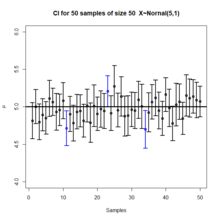
The coverage probability, , for Neyman construction is the frequency of experiments in which the confidence interval contains the actual value of interest. Generally, the coverage probability is set to a confidence. For Neyman construction, the coverage probability is set to some value where .
A Neyman construction can be carried out by performing multiple experiments that construct data sets corresponding to a given value of the parameter. The experiments are fitted with conventional methods, and the space of fitted parameter values constitutes the band which the confidence interval can be selected from.
Suppose , where and are unknown constants where we wish to estimate . We can define (2) single value functions, and , defined by the process above such that given a pre-specified confidence level, , and random sample
where is the standard error, and the sample mean and standard deviation are:
The factor follows a t distribution with (n-1) degrees of freedom, ~t [2]
are iid random variables, and let . Suppose . Now to construct a confidence interval with level of confidence. We know is sufficient for . So,
This produces a confidence interval for where,

In probability theory and statistics, the cumulative distribution function (CDF) of a real-valued random variable , or just distribution function of , evaluated at , is the probability that will take a value less than or equal to .
In probability theory, the central limit theorem (CLT) states that, under appropriate conditions, the distribution of a normalized version of the sample mean converges to a standard normal distribution. This holds even if the original variables themselves are not normally distributed. There are several versions of the CLT, each applying in the context of different conditions.
The likelihood function is the joint probability mass of observed data viewed as a function of the parameters of a statistical model. Intuitively, the likelihood function is the probability of observing data assuming is the actual parameter.

In probability theory and statistics, the chi-squared distribution with degrees of freedom is the distribution of a sum of the squares of independent standard normal random variables. The chi-squared distribution is a special case of the gamma distribution and is one of the most widely used probability distributions in inferential statistics, notably in hypothesis testing and in construction of confidence intervals. This distribution is sometimes called the central chi-squared distribution, a special case of the more general noncentral chi-squared distribution.
In statistics, maximum likelihood estimation (MLE) is a method of estimating the parameters of an assumed probability distribution, given some observed data. This is achieved by maximizing a likelihood function so that, under the assumed statistical model, the observed data is most probable. The point in the parameter space that maximizes the likelihood function is called the maximum likelihood estimate. The logic of maximum likelihood is both intuitive and flexible, and as such the method has become a dominant means of statistical inference.
In statistics, a statistic is sufficient with respect to a statistical model and its associated unknown parameter if "no other statistic that can be calculated from the same sample provides any additional information as to the value of the parameter". In particular, a statistic is sufficient for a family of probability distributions if the sample from which it is calculated gives no additional information than the statistic, as to which of those probability distributions is the sampling distribution.

In probability theory, the law of large numbers (LLN) is a mathematical theorem that states that the average of the results obtained from a large number of independent and identical random samples converges to the true value, if it exists. More formally, the LLN states that given a sample of independent and identically distributed values, the sample mean converges to the true mean.
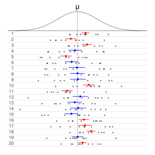
Informally, in frequentist statistics, a confidence interval (CI) is an interval which is expected to typically contain the parameter being estimated. More specifically, given a confidence level , a CI is a random interval which contains the parameter being estimated % of the time. The confidence level, degree of confidence or confidence coefficient represents the long-run proportion of CIs that theoretically contain the true value of the parameter; this is tantamount to the nominal coverage probability. For example, out of all intervals computed at the 95% level, 95% of them should contain the parameter's true value.
In statistics, the Neyman–Pearson lemma describes the existence and uniqueness of the likelihood ratio as a uniformly most powerful test in certain contexts. It was introduced by Jerzy Neyman and Egon Pearson in a paper in 1933. The Neyman–Pearson lemma is part of the Neyman–Pearson theory of statistical testing, which introduced concepts like errors of the second kind, power function, and inductive behavior. The previous Fisherian theory of significance testing postulated only one hypothesis. By introducing a competing hypothesis, the Neyman–Pearsonian flavor of statistical testing allows investigating the two types of errors. The trivial cases where one always rejects or accepts the null hypothesis are of little interest but it does prove that one must not relinquish control over one type of error while calibrating the other. Neyman and Pearson accordingly proceeded to restrict their attention to the class of all level tests while subsequently minimizing type II error, traditionally denoted by . Their seminal paper of 1933, including the Neyman–Pearson lemma, comes at the end of this endeavor, not only showing the existence of tests with the most power that retain a prespecified level of type I error, but also providing a way to construct such tests. The Karlin-Rubin theorem extends the Neyman–Pearson lemma to settings involving composite hypotheses with monotone likelihood ratios.

In statistics, a consistent estimator or asymptotically consistent estimator is an estimator—a rule for computing estimates of a parameter θ0—having the property that as the number of data points used increases indefinitely, the resulting sequence of estimates converges in probability to θ0. This means that the distributions of the estimates become more and more concentrated near the true value of the parameter being estimated, so that the probability of the estimator being arbitrarily close to θ0 converges to one.

In probability theory and statistics, the continuous uniform distributions or rectangular distributions are a family of symmetric probability distributions. Such a distribution describes an experiment where there is an arbitrary outcome that lies between certain bounds. The bounds are defined by the parameters, and which are the minimum and maximum values. The interval can either be closed or open. Therefore, the distribution is often abbreviated where stands for uniform distribution. The difference between the bounds defines the interval length; all intervals of the same length on the distribution's support are equally probable. It is the maximum entropy probability distribution for a random variable under no constraint other than that it is contained in the distribution's support.
In statistics, an exchangeable sequence of random variables is a sequence X1, X2, X3, ... whose joint probability distribution does not change when the positions in the sequence in which finitely many of them appear are altered. In other words, the joint distribution is invariant to finite permutation. Thus, for example the sequences
In estimation theory and decision theory, a Bayes estimator or a Bayes action is an estimator or decision rule that minimizes the posterior expected value of a loss function. Equivalently, it maximizes the posterior expectation of a utility function. An alternative way of formulating an estimator within Bayesian statistics is maximum a posteriori estimation.
A ratio distribution is a probability distribution constructed as the distribution of the ratio of random variables having two other known distributions. Given two random variables X and Y, the distribution of the random variable Z that is formed as the ratio Z = X/Y is a ratio distribution.
In statistical hypothesis testing, a uniformly most powerful (UMP) test is a hypothesis test which has the greatest power among all possible tests of a given size α. For example, according to the Neyman–Pearson lemma, the likelihood-ratio test is UMP for testing simple (point) hypotheses.

In probability theory and statistics, the Poisson distribution is a discrete probability distribution that expresses the probability of a given number of events occurring in a fixed interval of time if these events occur with a known constant mean rate and independently of the time since the last event. It can also be used for the number of events in other types of intervals than time, and in dimension greater than 1.
A product distribution is a probability distribution constructed as the distribution of the product of random variables having two other known distributions. Given two statistically independent random variables X and Y, the distribution of the random variable Z that is formed as the product is a product distribution.
In statistical inference, the concept of a confidence distribution (CD) has often been loosely referred to as a distribution function on the parameter space that can represent confidence intervals of all levels for a parameter of interest. Historically, it has typically been constructed by inverting the upper limits of lower sided confidence intervals of all levels, and it was also commonly associated with a fiducial interpretation, although it is a purely frequentist concept. A confidence distribution is NOT a probability distribution function of the parameter of interest, but may still be a function useful for making inferences.
Exponential Tilting (ET), Exponential Twisting, or Exponential Change of Measure (ECM) is a distribution shifting technique used in many parts of mathematics. The different exponential tiltings of a random variable is known as the natural exponential family of .


