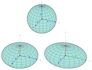
Orbital elements

Last updated May 10, 2024

Orbital elements are the parameters required to uniquely identify a specific orbit. In celestial mechanics these elements are considered in two-body systems using a Kepler orbit. There are many different ways to mathematically describe the same orbit, but certain schemes, each consisting of a set of six parameters, are commonly used in astronomy and orbital mechanics.

Keplerian elements

In this diagram, the orbital plane (yellow) intersects a reference plane (gray). For Earth-orbiting satellites, the reference plane is usually the Earth's equatorial plane, and for satellites in solar orbits it is the ecliptic plane. The intersection is called the line of nodes, as it connects the reference body (the primary) with the ascending and descending nodes. The reference body and the vernal point ([?]) establish a reference direction and, together with the reference plane, they establish a reference frame. Orbit1.svg — In this diagram, the orbital plane (yellow) intersects a reference plane (gray). For Earth-orbiting satellites, the reference plane is usually the Earth's equatorial plane, and for satellites in solar orbits it is the ecliptic plane. The intersection is called the line of nodes, as it connects the reference body (the primary) with the ascending and descending nodes. The reference body and the vernal point (♈︎) establish a reference direction and, together with the reference plane, they establish a reference frame.

The traditional orbital elements are the six Keplerian elements, after Johannes Kepler and his laws of planetary motion.

When viewed from an inertial frame, two orbiting bodies trace out distinct trajectories. Each of these trajectories has its focus at the common center of mass. When viewed from a non-inertial frame centered on one of the bodies, only the trajectory of the opposite body is apparent; Keplerian elements describe these non-inertial trajectories. An orbit has two sets of Keplerian elements depending on which body is used as the point of reference. The reference body (usually the most massive) is called the primary , the other body is called the secondary. The primary does not necessarily possess more mass than the secondary, and even when the bodies are of equal mass, the orbital elements depend on the choice of the primary.

Two elements define the shape and size of the ellipse:

Eccentricity ( $e$ )—shape of the ellipse, describing how much it is elongated compared to a circle (not marked in diagram).
Semi-major axis ( $a$ ) — half the distance between the apoapsis and periapsis. The portion of the semi-major axis extending from the primary at one focus to the periapsis is shown as a purple line in the diagram; the rest (from the primary/focus to the center of the orbit ellipse) is below the reference plane and not shown.

Two elements define the orientation of the orbital plane in which the ellipse is embedded:

Inclination ( $i$ ) — vertical tilt of the ellipse with respect to the reference plane, measured at the ascending node (where the orbit passes upward through the reference plane, the green angle $i$ in the diagram). Tilt angle is measured perpendicular to line of intersection between orbital plane and reference plane. Any three distinct points on an ellipse will define the ellipse orbital plane. The plane and the ellipse are both two-dimensional objects defined in three-dimensional space.
Longitude of the ascending node ( $Ω$ ) — horizontally orients the ascending node of the ellipse (where the orbit passes from south to north through the reference plane, symbolized by $☊$ ) with respect to the reference frame's vernal point (symbolized by ♈︎). This is measured in the reference plane, and is shown as the green angle $Ω$ in the diagram.

The remaining two elements are as follows:

Argument of periapsis ( $ω$ ) defines the orientation of the ellipse in the orbital plane, as an angle measured from the ascending node to the periapsis (the closest point the satellite body comes to the primary body around which it orbits), the purple angle $ω$ in the diagram.
True anomaly ( $ν$ , $θ$ , or $f$ ) at epoch ( $t 0$ ) defines the position of the orbiting body along the ellipse at a specific time (the "epoch").

The mean anomaly $M$ is a mathematically convenient fictitious "angle" which varies linearly with time, but which does not correspond to a real geometric angle. It can be converted into the true anomaly $ν$ , which does represent the real geometric angle in the plane of the ellipse, between periapsis (closest approach to the central body) and the position of the orbiting body at any given time. Thus, the true anomaly is shown as the red angle $ν$ in the diagram, and the mean anomaly is not shown.

The angles of inclination, longitude of the ascending node, and argument of periapsis can also be described as the Euler angles defining the orientation of the orbit relative to the reference coordinate system.

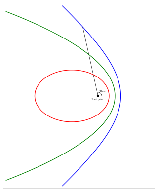
Note that non-elliptic trajectories also exist, but are not closed, and are thus not orbits. If the eccentricity is greater than one, the trajectory is a hyperbola. If the eccentricity is equal to one and the angular momentum is zero, the trajectory is radial. If the eccentricity is one and there is angular momentum, the trajectory is a parabola.

Required parameters

Given an inertial frame of reference and an arbitrary epoch (a specified point in time), exactly six parameters are necessary to unambiguously define an arbitrary and unperturbed orbit.

This is because the problem contains six degrees of freedom. These correspond to the three spatial dimensions which define position ( $x$ , $y$ , $z$ in a Cartesian coordinate system), plus the velocity in each of these dimensions. These can be described as orbital state vectors, but this is often an inconvenient way to represent an orbit, which is why Keplerian elements are commonly used instead.

Sometimes the epoch is considered a "seventh" orbital parameter, rather than part of the reference frame.

If the epoch is defined to be at the moment when one of the elements is zero, the number of unspecified elements is reduced to five. (The sixth parameter is still necessary to define the orbit; it is merely numerically set to zero by convention or "moved" into the definition of the epoch with respect to real-world clock time.)

Alternative parametrizations

Keplerian elements can be obtained from orbital state vectors (a three-dimensional vector for the position and another for the velocity) by manual transformations or with computer software.^[1]

Other orbital parameters can be computed from the Keplerian elements such as the period, apoapsis, and periapsis. (When orbiting the Earth, the last two terms are known as the apogee and perigee.) It is common to specify the period instead of the semi-major axis in Keplerian element sets, as each can be computed from the other provided the standard gravitational parameter, $GM$ , is given for the central body.

Instead of the mean anomaly at epoch, the mean anomaly $M$ , mean longitude, true anomaly $ν 0$ , or (rarely) the eccentric anomaly might be used.

Using, for example, the "mean anomaly" instead of "mean anomaly at epoch" means that time $t$ must be specified as a seventh orbital element. Sometimes it is assumed that mean anomaly is zero at the epoch (by choosing the appropriate definition of the epoch), leaving only the five other orbital elements to be specified.

Different sets of elements are used for various astronomical bodies. The eccentricity, $e$ , and either the semi-major axis, $a$ , or the distance of periapsis, $q$ , are used to specify the shape and size of an orbit. The longitude of the ascending node, $Ω$ , the inclination, $i$ , and the argument of periapsis, $ω$ , or the longitude of periapsis, $ϖ$ , specify the orientation of the orbit in its plane. Either the longitude at epoch, $L 0$ , the mean anomaly at epoch, $M 0$ , or the time of perihelion passage, $T 0$ , are used to specify a known point in the orbit. The choices made depend whether the vernal equinox or the node are used as the primary reference. The semi-major axis is known if the mean motion and the gravitational mass are known.^[2]^[3]

It is also quite common to see either the mean anomaly ( $M$ ) or the mean longitude ( $L$ ) expressed directly, without either $M 0$ or $L 0$ as intermediary steps, as a polynomial function with respect to time. This method of expression will consolidate the mean motion ( $n$ ) into the polynomial as one of the coefficients. The appearance will be that $L$ or $M$ are expressed in a more complicated manner, but we will appear to need one fewer orbital element.

Mean motion can also be obscured behind citations of the orbital period $P$ .^{[ clarification needed ]}

Sets of orbital elements
Object	Elements used
Major planet	$e, a, i, Ω, ϖ, L 0$
Comet	$e, q, i, Ω, ω, T 0$
Asteroid	$e, a, i, Ω, ω, M 0$
Two-line elements	$e, i, Ω, ω, n, M 0$

Euler angle transformations

The angles $Ω$ , $i$ , $ω$ are the Euler angles (corresponding to $α$ , $β$ , $γ$ in the notation used in that article) characterizing the orientation of the coordinate system

$x̂$ , $ŷ$ , $ẑ$ from the inertial coordinate frame $Î$ , $Ĵ$ , $K̂$

where:

$Î$ , $Ĵ$ is in the equatorial plane of the central body. $Î$ is in the direction of the vernal equinox. $Ĵ$ is perpendicular to $Î$ and with $Î$ defines the reference plane. $K̂$ is perpendicular to the reference plane. Orbital elements of bodies (planets, comets, asteroids, ...) in the Solar System usually the ecliptic as that plane.
$x̂$ , $ŷ$ are in the orbital plane and with $x̂$ in the direction to the pericenter (periapsis). $ẑ$ is perpendicular to the plane of the orbit. $ŷ$ is mutually perpendicular to $x̂$ and $ẑ$ .

Then, the transformation from the $Î$ , $Ĵ$ , $K̂$ coordinate frame to the $x̂$ , $ŷ$ , $ẑ$ frame with the Euler angles $Ω$ , $i$ , $ω$ is:

{\displaystyle {\begin{aligned}x_{1}&=\cos \Omega \cdot \cos \omega -\sin \Omega \cdot \cos i\cdot \sin \omega \

{\begin{bmatrix}x_{1}&x_{2}&x_{3}\\y_{1}&y_{2}&y_{3}\\z_{1}&z_{2}&z_{3}\end{bmatrix}}={\begin{bmatrix}\cos \omega &\sin \omega &0\\-\sin \omega &\cos \omega &0\\0&0&1\end{bmatrix}}\,{\begin{bmatrix}1&0&0\\0&\cos i&\sin i\\0&-\sin i&\cos i\end{bmatrix}}\,{\begin{bmatrix}\cos \Omega &\sin \Omega &0\\-\sin \Omega &\cos \Omega &0\\0&0&1\end{bmatrix}}\,;

where

{\begin{aligned}\mathbf {\hat {x}} &=x_{1}\mathbf {\hat {I}} +x_{2}\mathbf {\hat {J}} +x_{3}\mathbf {\hat {K}} ~;\\\mathbf {\hat {y}} &=y_{1}\mathbf {\hat {I}} +y_{2}\mathbf {\hat {J}} +y_{3}\mathbf {\hat {K}} ~;\\\mathbf {\hat {z}} &=z_{1}\mathbf {\hat {I}} +z_{2}\mathbf {\hat {J}} +z_{3}\mathbf {\hat {K}} ~.\\\end{aligned}}

The inverse transformation, which computes the 3 coordinates in the I-J-K system given the 3 (or 2) coordinates in the x-y-z system, is represented by the inverse matrix. According to the rules of matrix algebra, the inverse matrix of the product of the 3 rotation matrices is obtained by inverting the order of the three matrices and switching the signs of the three Euler angles.

That is,

{\begin{bmatrix}i_{1}&i_{2}&i_{3}\\j_{1}&j_{2}&j_{3}\\k_{1}&k_{2}&k_{3}\end{bmatrix}}={\begin{bmatrix}\cos \Omega &-\sin \Omega &0\\\sin \Omega &\cos \Omega &0\\0&0&1\end{bmatrix}}\,{\begin{bmatrix}1&0&0\\0&\cos i&-\sin i\\0&\sin i&\cos i\end{bmatrix}}\,{\begin{bmatrix}\cos \omega &-\sin \omega &0\\\sin \omega &\cos \omega &0\\0&0&1\end{bmatrix}}\,;

where

{\begin{aligned}\mathbf {\hat {I}} &=i_{1}\mathbf {\hat {x}} +i_{2}\mathbf {\hat {y}} +i_{3}\mathbf {\hat {z}} ~;\\\mathbf {\hat {J}} &=j_{1}\mathbf {\hat {x}} +j_{2}\mathbf {\hat {y}} +j_{3}\mathbf {\hat {z}} ~;\\\mathbf {\hat {K}} &=k_{1}\mathbf {\hat {x}} +k_{2}\mathbf {\hat {y}} +k_{3}\mathbf {\hat {z}} ~.\\\end{aligned}}

The transformation from $x̂$ , $ŷ$ , $ẑ$ to Euler angles $Ω$ , $i$ , $ω$ is:

{\begin{aligned}\Omega &=\operatorname {arg} \left(-z_{2},z_{1}\right)\\i&=\operatorname {arg} \left(z_{3},{\sqrt {{z_{1}}^{2}+{z_{2}}^{2}}}\right)\\\omega &=\operatorname {arg} \left(y_{3},x_{3}\right)\\\end{aligned}}

where $arg(x, y)$ signifies the polar argument that can be computed with the standard function atan2(y,x) available in many programming languages.

Orbit prediction

Under ideal conditions of a perfectly spherical central body, zero perturbations and negligible relativistic effects, all orbital elements except the mean anomaly are constants. The mean anomaly changes linearly with time, scaled by the mean motion,^[2]

n={\sqrt {\frac {\mu }{a^{3}}}}.

where $μ$ is the standard gravitational parameter. Hence if at any instant $t 0$ the orbital parameters are $(e 0, a 0, i 0, Ω 0, ω 0, M 0)$ , then the elements at time $t = t 0 + δt$ is given by $(e 0, a 0, i 0, Ω 0, ω 0, M 0 + n δt)$

Perturbations and elemental variance

Unperturbed, two-body, Newtonian orbits are always conic sections, so the Keplerian elements define an ellipse, parabola, or hyperbola. Real orbits have perturbations, so a given set of Keplerian elements accurately describes an orbit only at the epoch. Evolution of the orbital elements takes place due to the gravitational pull of bodies other than the primary, the nonsphericity of the primary, atmospheric drag, relativistic effects, radiation pressure, electromagnetic forces, and so on.

Keplerian elements can often be used to produce useful predictions at times near the epoch. Alternatively, real trajectories can be modeled as a sequence of Keplerian orbits that osculate ("kiss" or touch) the real trajectory. They can also be described by the so-called planetary equations, differential equations which come in different forms developed by Lagrange, Gauss, Delaunay, Poincaré, or Hill.

Two-line elements

Keplerian elements parameters can be encoded as text in a number of formats. The most common of them is the NASA / NORAD "two-line elements" (TLE) format,^[4] originally designed for use with 80 column punched cards, but still in use because it is the most common format, and can be handled easily by all modern data storages as well.

Depending on the application and object orbit, the data derived from TLEs older than 30 days can become unreliable. Orbital positions can be calculated from TLEs through the SGP / SGP4 / SDP4 / SGP8 / SDP8 algorithms.^[5]

Example of a two-line element:^[6]

1 27651U 03004A   07083.49636287  .00000119  00000-0  30706-4 0  2692 2 27651 039.9951 132.2059 0025931 073.4582 286.9047 14.81909376225249

Delaunay variables

The Delaunay orbital elements were introduced by Charles-Eugène Delaunay during his study of the motion of the Moon.^[7] Commonly called Delaunay variables, they are a set of canonical variables, which are action-angle coordinates. The angles are simple sums of some of the Keplerian angles:

the mean longitude: $\ell =M+\omega +\Omega \,,$
the longitude of periapsis: $g=\omega +\Omega \,,$ and
the longitude of the ascending node: $h=\Omega$

along with their respective conjugate momenta, $L$ , $G$ , and $H$ .^[8] The momenta $L$ , $G$ , and $H$ are the action variables and are more elaborate combinations of the Keplerian elements $a$ , $e$ , and $i$ .

Delaunay variables are used to simplify perturbative calculations in celestial mechanics, for example while investigating the Kozai–Lidov oscillations in hierarchical triple systems.^[8] The advantage of the Delaunay variables is that they remain well defined and non-singular (except for $h$ , which can be tolerated) when $e$ and / or $i$ are very small: When the test particle's orbit is very nearly circular ( $e\approx 0$ ), or very nearly “flat” ( $i\approx 0$ ).

Related Research Articles

In astronomy, Kepler's laws of planetary motion, published by Johannes Kepler between 1609 and 1619, describe the orbits of planets around the Sun. The laws modified the heliocentric theory of Nicolaus Copernicus, replacing its circular orbits and epicycles with elliptical trajectories, and explaining how planetary velocities vary. The three laws state that:

The orbit of a planet is an ellipse with the Sun at one of the two foci.
A line segment joining a planet and the Sun sweeps out equal areas during equal intervals of time.
The square of a planet's orbital period is proportional to the cube of the length of the semi-major axis of its orbit.

In celestial mechanics, an orbit is the curved trajectory of an object such as the trajectory of a planet around a star, or of a natural satellite around a planet, or of an artificial satellite around an object or position in space such as a planet, moon, asteroid, or Lagrange point. Normally, orbit refers to a regularly repeating trajectory, although it may also refer to a non-repeating trajectory. To a close approximation, planets and satellites follow elliptic orbits, with the center of mass being orbited at a focal point of the ellipse, as described by Kepler's laws of planetary motion.

In mathematics, a spherical coordinate system is a coordinate system for three-dimensional space where the position of a given point in space is specified by three numbers, : the radial distance of the radial liner connecting the point to the fixed point of origin ; the polar angle θ of the radial line r; and the azimuthal angle φ of the radial line r.

Kinematics is a subfield of physics and mathematics, developed in classical mechanics, that describes the motion of points, bodies (objects), and systems of bodies without considering the forces that cause them to move. Kinematics, as a field of study, is often referred to as the "geometry of motion" and is occasionally seen as a branch of both applied and pure mathematics since it can be studied without considering the mass of a body or the forces acting upon it. A kinematics problem begins by describing the geometry of the system and declaring the initial conditions of any known values of position, velocity and/or acceleration of points within the system. Then, using arguments from geometry, the position, velocity and acceleration of any unknown parts of the system can be determined. The study of how forces act on bodies falls within kinetics, not kinematics. For further details, see analytical dynamics.

<span class="mw-page-title-main">Angular velocity</span> Direction and rate of rotation

In physics, angular velocity, also known as angular frequency vector, is a pseudovector representation of how the angular position or orientation of an object changes with time, i.e. how quickly an object rotates around an axis of rotation and how fast the axis itself changes direction.

<span class="mw-page-title-main">Ellipsoid</span> Quadric surface that looks like a deformed sphere

An ellipsoid is a surface that can be obtained from a sphere by deforming it by means of directional scalings, or more generally, of an affine transformation.

In mechanics and geometry, the 3D rotation group, often denoted SO(3), is the group of all rotations about the origin of three-dimensional Euclidean space $under the operation of composition.$

An infinitesimal rotation matrix or differential rotation matrix is a matrix representing an infinitely small rotation.

In linear algebra, linear transformations can be represented by matrices. If $is a linear transformation mapping to and is a column vector with entries, then$

In celestial mechanics, true anomaly is an angular parameter that defines the position of a body moving along a Keplerian orbit. It is the angle between the direction of periapsis and the current position of the body, as seen from the main focus of the ellipse.

Screw theory is the algebraic calculation of pairs of vectors, such as angular and linear velocity, or forces and moments, that arise in the kinematics and dynamics of rigid bodies.

Spacecraft flight dynamics is the application of mechanical dynamics to model how the external forces acting on a space vehicle or spacecraft determine its flight path. These forces are primarily of three types: propulsive force provided by the vehicle's engines; gravitational force exerted by the Earth and other celestial bodies; and aerodynamic lift and drag.

In geometry, the circumscribed circle or circumcircle of a triangle is a circle that passes through all three vertices. The center of this circle is called the circumcenter of the triangle, and its radius is called the circumradius. The circumcenter is the point of intersection between the three perpendicular bisectors of the triangle's sides, and is a triangle center.

In mathematics, the Weierstrass–Enneper parameterization of minimal surfaces is a classical piece of differential geometry.

The perifocal coordinate (PQW) system is a frame of reference for an orbit. The frame is centered at the focus of the orbit, i.e. the celestial body about which the orbit is centered. The unit vectors $and lie in the plane of the orbit. is directed towards the periapsis of the orbit and has a true anomaly of 90 degrees past the periapsis. The third unit vector is the angular momentum vector and is directed orthogonal to the orbital plane such that:$

In geometry, various formalisms exist to express a rotation in three dimensions as a mathematical transformation. In physics, this concept is applied to classical mechanics where rotational kinematics is the science of quantitative description of a purely rotational motion. The orientation of an object at a given instant is described with the same tools, as it is defined as an imaginary rotation from a reference placement in space, rather than an actually observed rotation from a previous placement in space.

Orbit determination is the estimation of orbits of objects such as moons, planets, and spacecraft. One major application is to allow tracking newly observed asteroids and verify that they have not been previously discovered. The basic methods were discovered in the 17th century and have been continuously refined.

In mathematics, the axis–angle representation parameterizes a rotation in a three-dimensional Euclidean space by two quantities: a unit vector $e$ indicating the direction (geometry) of an axis of rotation, and an angle of rotation $θ$ describing the magnitude and sense of the rotation about the axis. Only two numbers, not three, are needed to define the direction of a unit vector $e$ rooted at the origin because the magnitude of $e$ is constrained. For example, the elevation and azimuth angles of $e$ suffice to locate it in any particular Cartesian coordinate frame.

In celestial mechanics, a Kepler orbit is the motion of one body relative to another, as an ellipse, parabola, or hyperbola, which forms a two-dimensional orbital plane in three-dimensional space. A Kepler orbit can also form a straight line. It considers only the point-like gravitational attraction of two bodies, neglecting perturbations due to gravitational interactions with other objects, atmospheric drag, solar radiation pressure, a non-spherical central body, and so on. It is thus said to be a solution of a special case of the two-body problem, known as the Kepler problem. As a theory in classical mechanics, it also does not take into account the effects of general relativity. Keplerian orbits can be parametrized into six orbital elements in various ways.

The direct-quadrature-zerotransformation or zero-direct-quadraturetransformation is a tensor that rotates the reference frame of a three-element vector or a three-by-three element matrix in an effort to simplify analysis. The DQZ transform is the product of the Clarke transform and the Park transform, first proposed in 1929 by Robert H. Park.

References

↑ For example, with "VEC2TLE". amsat.org. Archived from the original on 20 May 2016. Retrieved 19 June 2013.
1 2 Green, Robin M. (1985). Spherical Astronomy. Cambridge University Press. ISBN 978-0-521-23988-2.
↑ Danby, J.M.A. (1962). Fundamentals of Celestial Mechanics. Willmann-Bell. ISBN 978-0-943396-20-0.
↑ Kelso, T.S. "FAQs: Two-line element set format". celestrak.com. CelesTrak. Archived from the original on 26 March 2016. Retrieved 15 June 2016.
↑ Seidelmann, K.P., ed. (1992). Explanatory Supplement to the Astronomical Almanac (1st ed.). Mill Valley, CA: University Science Books.
↑ "SORCE". Heavens-Above.com. orbit data. Archived from the original on 27 September 2007.
↑ Aubin, David (2014). "Delaunay, Charles-Eugène". Biographical Encyclopedia of Astronomers. New York, NY: Springer New York. pp. 548–549. doi:10.1007/978-1-4419-9917-7_347. ISBN 978-1-4419-9916-0.
1 2 Shevchenko, Ivan (2017). The Lidov–Kozai effect: applications in exoplanet research and dynamical astronomy. Cham: Springer. ISBN 978-3-319-43522-0.

External links

Gurfil, Pini (2005). "Euler parameters as nonsingular orbital elements in Near-Equatorial Orbits". Journal of Guidance, Control, and Dynamics. 28 (5): 1079–1084. Bibcode:2005JGCD...28.1079G. doi:10.2514/1.14760.

"Tutorial". AMSAT . Keplerian elements. Archived from the original on 14 October 2002.

"Orbits Tutorial". marine.rutgers.edu. Archived from the original on 19 April 2021. Retrieved 30 July 2019.

"Orbital elements visualizer". orbitalmechanics.info.

Report No. 3 (PDF). celestrak (Report). Spacetrack. North American Aerospace Defense Command (NORAD). Archived (PDF) from the original on 3 September 2000. – a serious treatment of orbital elements

"FAQ". Celestrak. Two-Line Elements. Archived from the original on 26 March 2016.

"The JPL HORIZONS online ephemeris". – also furnishes orbital elements for a large number of solar system objects

"Mean orbital parameters". ssd.jpl.nasa.gov. Planetary satellites. JPL / NASA.

"Introduction to exporting". ssd.jpl.nasa.gov. JPL planetary and lunar ephemerides. JPL / NASA.

"State vectors: VEC2TLE". MindSpring (software). Archived from the original on 3 March 2016. – access to VEC2TLE software

"Function 'iauPlan94'" (C software source). IAU SOFA C Library. – orbital elements of the major planets

This page is based on this Wikipedia article
Text is available under the CC BY-SA 4.0 license; additional terms may apply.
Images, videos and audio are available under their respective licenses.

[1] For example, with "VEC2TLE". amsat.org. Archived from the original on 20 May 2016. Retrieved 19 June 2013.

[Green-2] 1 2 Green, Robin M. (1985). Spherical Astronomy. Cambridge University Press. ISBN 978-0-521-23988-2.

[Danby-3] Danby, J.M.A. (1962). Fundamentals of Celestial Mechanics. Willmann-Bell. ISBN 978-0-943396-20-0.

[Kelso_FAQ-4] Kelso, T.S. "FAQs: Two-line element set format". celestrak.com. CelesTrak. Archived from the original on 26 March 2016. Retrieved 15 June 2016.

[5] Seidelmann, K.P., ed. (1992). Explanatory Supplement to the Astronomical Almanac (1st ed.). Mill Valley, CA: University Science Books.

[6] "SORCE". Heavens-Above.com. orbit data. Archived from the original on 27 September 2007.

[Aubin-2014-7] Aubin, David (2014). "Delaunay, Charles-Eugène". Biographical Encyclopedia of Astronomers. New York, NY: Springer New York. pp. 548–549. doi:10.1007/978-1-4419-9917-7_347. ISBN 978-1-4419-9916-0.

[Shevchenko-2017-8] 1 2 Shevchenko, Ivan (2017). The Lidov–Kozai effect: applications in exoplanet research and dynamical astronomy. Cham: Springer. ISBN 978-3-319-43522-0.

[1]

[2]

[3]

[4]

[5]

[6]

[7]

[8]