Petri net

A Petri net, also known as a place/transition net (PT net), is one of several mathematical modeling languages for the description of distributed systems. It is a class of discrete event dynamic system. A Petri net is a directed bipartite graph that has two types of elements: places and transitions. Place elements are depicted as white circles and transition elements are depicted as rectangles. A place can contain any number of tokens, depicted as black circles. A transition is enabled if all places connected to it as inputs contain at least one token. Some sources ^[1] state that Petri nets were invented in August 1939 by Carl Adam Petri—at the age of 13—for the purpose of describing chemical processes.

Like industry standards such as UML activity diagrams, Business Process Model and Notation, and event-driven process chains, Petri nets offer a graphical notation for stepwise processes that include choice, iteration, and concurrent execution. Unlike these standards, Petri nets have an exact mathematical definition of their execution semantics, with a well-developed mathematical theory for process analysis^{[ citation needed ]}.

(a) Petri net trajectory example

Historical background

The German computer scientist Carl Adam Petri, after whom such structures are named, analyzed Petri nets extensively in his 1962 dissertation Kommunikation mit Automaten.

Petri net basics

A Petri net consists of places, transitions, and arcs . Arcs run from a place to a transition or vice versa, never between places or between transitions. The places from which an arc runs to a transition are called the input places of the transition; the places to which arcs run from a transition are called the output places of the transition.

Graphically, places in a Petri net may contain a discrete number of marks called tokens. Any distribution of tokens over the places will represent a configuration of the net called a marking. In an abstract sense relating to a Petri net diagram, a transition of a Petri net may fire if it is enabled, i.e. there are sufficient tokens in all of its input places; when the transition fires, it consumes the required input tokens, and creates tokens in its output places. A firing is atomic, i.e. a single non-interruptible step.

Unless an execution policy (e.g. a strict ordering of transitions, describing precedence) is defined, the execution of Petri nets is nondeterministic: when multiple transitions are enabled at the same time, they will fire in any order.

Since firing is nondeterministic, and multiple tokens may be present anywhere in the net (even in the same place), Petri nets are well suited for modeling the concurrent behavior of distributed systems.

Formal definition and basic terminology

Petri nets are state-transition systems that extend a class of nets called elementary nets. ^[2]

Definition 1. A net is a tuple ${\displaystyle N=(P,T,F)}$ where

1. ${\displaystyle P}$ and ${\displaystyle T}$ are disjoint finite sets of places and transitions, respectively.
2. ${\displaystyle F\subseteq (P\times T)\cup (T\times P)}$ is a set of (directed) arcs (or flow relations).

Definition 2. Given a net N = (P, T, F), a configuration is a set C so that C⊆P.

A Petri net with an enabled transition.

The Petri net that follows after the transition fires (Initial Petri net in the figure above).

Definition 3. An elementary net is a net of the form EN = (N, C) where

1. N = (P, T, F) is a net.
2. C is such that C⊆P is a configuration.

Definition 4. A Petri net is a net of the form PN = (N, M, W), which extends the elementary net so that

1. N = (P, T, F) is a net.
2. M : P→Z is a place multiset, where Z is a countable set. M extends the concept of configuration and is commonly described with reference to Petri net diagrams as a marking.
3. W : F→Z is an arc multiset, so that the count (or weight) for each arc is a measure of the arc multiplicity.

If a Petri net is equivalent to an elementary net, then Z can be the countable set {0,1} and those elements in P that map to 1 under M form a configuration. Similarly, if a Petri net is not an elementary net, then the multiset M can be interpreted as representing a non-singleton set of configurations. In this respect, M extends the concept of configuration for elementary nets to Petri nets.

In the diagram of a Petri net (see top figure right), places are conventionally depicted with circles, transitions with long narrow rectangles and arcs as one-way arrows that show connections of places to transitions or transitions to places. If the diagram were of an elementary net, then those places in a configuration would be conventionally depicted as circles, where each circle encompasses a single dot called a token. In the given diagram of a Petri net (see right), the place circles may encompass more than one token to show the number of times a place appears in a configuration. The configuration of tokens distributed over an entire Petri net diagram is called a marking.

In the top figure (see right), the place p₁ is an input place of transition t; whereas, the place p₂ is an output place to the same transition. Let PN₀ (top figure) be a Petri net with a marking configured M₀, and PN₁ (bottom figure) be a Petri net with a marking configured M₁. The configuration of PN₀enables transition t through the property that all input places have sufficient number of tokens (shown in the figures as dots) "equal to or greater" than the multiplicities on their respective arcs to t. Once and only once a transition is enabled will the transition fire. In this example, the firing of transition t generates a map that has the marking configured M₁ in the image of M₀ and results in Petri net PN₁, seen in the bottom figure. In the diagram, the firing rule for a transition can be characterised by subtracting a number of tokens from its input places equal to the multiplicity of the respective input arcs and accumulating a new number of tokens at the output places equal to the multiplicity of the respective output arcs.

Remark 1. The precise meaning of "equal to or greater" will depend on the precise algebraic properties of addition being applied on Z in the firing rule, where subtle variations on the algebraic properties can lead to other classes of Petri nets; for example, algebraic Petri nets. ^[3]

The following formal definition is loosely based on ( Peterson 1981 ). Many alternative definitions exist.

Syntax

A Petri net graph (called Petri net by some, but see below) is a 3-tuple ${\displaystyle (S,T,W)}$, where

• S is a finite set of places
• T is a finite set of transitions
• S and T are disjoint, i.e. no object can be both a place and a transition
• ${\displaystyle W:(S\times T)\cup (T\times S)\to \mathbb {N} }$ is a multiset of arcs, i.e. it assigns to each arc a non-negative integer arc multiplicity (or weight); note that no arc may connect two places or two transitions.

The flow relation is the set of arcs: ${\displaystyle F=\{(x,y)\mid W(x,y)>0\}}$. In many textbooks, arcs can only have multiplicity 1. These texts often define Petri nets using F instead of W. When using this convention, a Petri net graph is a bipartite directed graph ${\displaystyle (S\cup T,F)}$ with node partitions S and T.

The preset of a transition t is the set of its input places: ${\displaystyle {}^{\bullet }t=\{s\in S\mid W(s,t)>0\}}$; its postset is the set of its output places: ${\displaystyle t^{\bullet }=\{s\in S\mid W(t,s)>0\}}$. Definitions of pre- and postsets of places are analogous.

A marking of a Petri net (graph) is a multiset of its places, i.e., a mapping ${\displaystyle M:S\to \mathbb {N} }$. We say the marking assigns to each place a number of tokens.

A Petri net (called marked Petri net by some, see above) is a 4-tuple ${\displaystyle (S,T,W,M_{0})}$, where

• ${\displaystyle (S,T,W)}$ is a Petri net graph;
• ${\displaystyle M_{0}}$ is the initial marking, a marking of the Petri net graph.

Execution semantics

In words

• firing a transition t in a marking M consumes ${\displaystyle W(s,t)}$ tokens from each of its input places s, and produces ${\displaystyle W(t,s)}$ tokens in each of its output places s
• a transition is enabled (it may fire) in M if there are enough tokens in its input places for the consumptions to be possible, i.e. if and only if ${\displaystyle \forall s:M(s)\geq W(s,t)}$.

We are generally interested in what may happen when transitions may continually fire in arbitrary order.

We say that a marking M'is reachable from a marking Min one step if ${\displaystyle M{\underset {G}{\longrightarrow }}M'}$; we say that it is reachable from M if ${\displaystyle M{\overset {*}{\underset {G}{\longrightarrow }}}M'}$, where ${\displaystyle {\overset {*}{\underset {G}{\longrightarrow }}}}$ is the reflexive transitive closure of ${\displaystyle {\underset {G}{\longrightarrow }}}$; that is, if it is reachable in 0 or more steps.

For a (marked) Petri net ${\displaystyle N=(S,T,W,M_{0})}$, we are interested in the firings that can be performed starting with the initial marking ${\displaystyle M_{0}}$. Its set of reachable markings is the set ${\displaystyle R(N)\ {\stackrel {D}{=}}\ \left\{M'{\Bigg |}M_{0}{\xrightarrow[{(S,T,W)}]{*}}M'\right\}}$

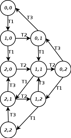
The reachability graph of N is the transition relation ${\displaystyle {\underset {G}{\longrightarrow }}}$ restricted to its reachable markings ${\displaystyle R(N)}$. It is the state space of the net.

A firing sequence for a Petri net with graph G and initial marking ${\displaystyle M_{0}}$ is a sequence of transitions ${\displaystyle {\vec {\sigma }}=\langle t_{1}\cdots t_{n}\rangle }$ such that ${\displaystyle M_{0}{\underset {G,t_{1}}{\longrightarrow }}M_{1}\wedge \cdots \wedge M_{n-1}{\underset {G,t_{n}}{\longrightarrow }}M_{n}}$. The set of firing sequences is denoted as ${\displaystyle L(N)}$.

Variations on the definition

A common variation is to disallow arc multiplicities and replace the bag of arcs W with a simple set, called the flow relation, ${\displaystyle F\subseteq (S\times T)\cup (T\times S)}$. This does not limit expressive power as both can represent each other.

Another common variation, e.g. in Desel and Juhás (2001), ^[4] is to allow capacities to be defined on places. This is discussed under extensions below.

Formulation in terms of vectors and matrices

The markings of a Petri net ${\displaystyle (S,T,W,M_{0})}$ can be regarded as vectors of non-negative integers of length ${\displaystyle |S|}$.

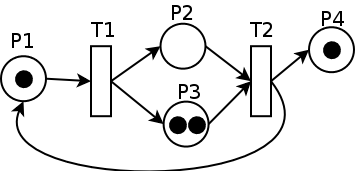
(b) Petri net example

Its transition relation can be described as a pair of ${\displaystyle |S|}$ by ${\displaystyle |T|}$ matrices:

• ${\displaystyle W^{-}}$, defined by ${\displaystyle \forall s,t:W^{-}[s,t]=W(s,t)}$
• ${\displaystyle W^{+}}$, defined by ${\displaystyle \forall s,t:W^{+}[s,t]=W(t,s).}$

Then their difference

• ${\displaystyle W^{T}=-W^{-}+W^{+}}$

can be used to describe the reachable markings in terms of matrix multiplication, as follows. For any sequence of transitions w, write ${\displaystyle o(w)}$ for the vector that maps every transition to its number of occurrences in w. Then, we have

• ${\displaystyle R(N)=\{M\mid \exists w:\ w{\text{ is a firing sequence of }}N\ {\text{ and }}\ M=M_{0}+W^{T}\cdot o(w)\}}$.

It must be required that w is a firing sequence; allowing arbitrary sequences of transitions will generally produce a larger set.

$${\displaystyle W^{-}={\begin{bmatrix}*&t1&t2\\p1&1&0\\p2&0&1\\p3&0&1\\p4&0&0\end{bmatrix}},\ W^{+}={\begin{bmatrix}*&t1&t2\\p1&0&1\\p2&1&0\\p3&1&0\\p4&0&1\end{bmatrix}},\ W^{T}={\begin{bmatrix}*&t1&t2\\p1&-1&1\\p2&1&-1\\p3&1&-1\\p4&0&1\end{bmatrix}}}$$

$${\displaystyle M_{0}={\begin{bmatrix}1&0&2&1\end{bmatrix}}}$$

Category-theoretic formulation

Meseguer and Montanari considered a kind of symmetric monoidal categories known as Petri categories. ^[5]

Mathematical properties of Petri nets

One thing that makes Petri nets interesting is that they provide a balance between modeling power and analyzability: many things one would like to know about concurrent systems can be automatically determined for Petri nets, although some of those things are very expensive to determine in the general case. Several subclasses of Petri nets have been studied that can still model interesting classes of concurrent systems, while these determinations become easier.

An overview of such decision problems, with decidability and complexity results for Petri nets and some subclasses, can be found in Esparza and Nielsen (1995). ^[6]

Reachability

The reachability problem for Petri nets is to decide, given a Petri net N and a marking M, whether ${\displaystyle M\in R(N)}$.

It is a matter of walking the reachability-graph defined above, until either the requested-marking is reached or it can no longer be found. This is harder than it may seem at first: the reachability graph is generally infinite, and it isn't easy to determine when it is safe to stop.

In fact, this problem was shown to be EXPSPACE-hard ^[7] years before it was shown to be decidable at all (Mayr, 1981). Papers continue to be published on how to do it efficiently. ^[8] In 2018, Czerwiński et al. improved the lower bound and showed that the problem is not ELEMENTARY. ^[9] In 2021, this problem was shown to be non-primitive recursive, independently by Jerome Leroux ^[10] and by Wojciech Czerwiński and Łukasz Orlikowski. ^[11] These results thus close the long-standing complexity gap.

While reachability seems to be a good tool to find erroneous states, for practical problems the constructed graph usually has far too many states to calculate. To alleviate this problem, linear temporal logic is usually used in conjunction with the tableau method to prove that such states cannot be reached. Linear temporal logic uses the semi-decision technique to find if indeed a state can be reached, by finding a set of necessary conditions for the state to be reached then proving that those conditions cannot be satisfied.

Liveness

A Petri net in which transition ${\displaystyle t_{0}}$ is dead, while for all ${\displaystyle j>0,}$${\displaystyle t_{j}}$ is ${\displaystyle L_{j}}$-live

Petri nets can be described as having different degrees of liveness ${\displaystyle L_{1}-L_{4}}$. A Petri net ${\displaystyle (N,M_{0})}$ is called ${\displaystyle L_{k}}$-live if and only if all of its transitions are ${\displaystyle L_{k}}$-live, where a transition is

• dead, if it can never fire, i.e. it is not in any firing sequence in ${\displaystyle L(N,M_{0})}$
• ${\displaystyle L_{1}}$-live (potentially fireable), if and only if it may fire, i.e. it is in some firing sequence in ${\displaystyle L(N,M_{0})}$
• ${\displaystyle L_{2}}$-live if it can fire arbitrarily often, i.e. if for every positive integer k, it occurs at least k times in some firing sequence in ${\displaystyle L(N,M_{0})}$
• ${\displaystyle L_{3}}$-live if it can fire infinitely often, i.e. if there is some fixed (necessarily infinite) firing sequence in which for every positive integer k, the transition ${\displaystyle L_{3}}$ occurs at least k times,
• ${\displaystyle L_{4}}$-live (live) if it may always fire, i.e. it is ${\displaystyle L_{1}}$-live in every reachable marking in ${\displaystyle R(N,M_{0})}$

Note that these are increasingly stringent requirements: ${\displaystyle L_{j+1}}$-liveness implies ${\displaystyle L_{j}}$-liveness, for ${\textstyle \textstyle {j\in {1,2,3}}}$.

These definitions are in accordance with Murata's overview, ^[12] which additionally uses ${\displaystyle L_{0}}$-live as a term for dead.

Boundedness

The reachability graph of N2.

A place in a Petri net is called k-bound if it does not contain more than k tokens in all reachable markings, including the initial marking; it is said to be safe if it is 1-bounded; it is bounded if it is k-bounded for some k.

A (marked) Petri net is called k-bounded, safe, or bounded when all of its places are. A Petri net (graph) is called (structurally) bounded if it is bounded for every possible initial marking.

A Petri net is bounded if and only if its reachability graph is finite.

Boundedness is decidable by looking at covering, by constructing the Karp–Miller Tree.

It can be useful to explicitly impose a bound on places in a given net. This can be used to model limited system resources.

Some definitions of Petri nets explicitly allow this as a syntactic feature. ^[13] Formally, Petri nets with place capacities can be defined as tuples ${\displaystyle (S,T,W,C,M_{0})}$, where ${\displaystyle (S,T,W,M_{0})}$ is a Petri net, ${\displaystyle C:P\rightarrow \!\!\!\shortmid \mathbb {N} }$ an assignment of capacities to (some or all) places, and the transition relation is the usual one restricted to the markings in which each place with a capacity has at most that many tokens.

An unbounded Petri net, N.

For example, if in the net N, both places are assigned capacity 2, we obtain a Petri net with place capacities, say N2; its reachability graph is displayed on the right.

A two-bounded Petri net, obtained by extending N with "counter-places".

Alternatively, places can be made bounded by extending the net. To be exact, a place can be made k-bounded by adding a "counter-place" with flow opposite to that of the place, and adding tokens to make the total in both places k.

Discrete, continuous, and hybrid Petri nets

As well as for discrete events, there are Petri nets for continuous and hybrid discrete-continuous processes ^[14] that are useful in discrete, continuous and hybrid control theory, ^[15] and related to discrete, continuous and hybrid automata.

Extensions

There are many extensions to Petri nets. Some of them are completely backwards-compatible (e.g. coloured Petri nets) with the original Petri net, some add properties that cannot be modelled in the original Petri net formalism (e.g. timed Petri nets). Although backwards-compatible models do not extend the computational power of Petri nets, they may have more succinct representations and may be more convenient for modeling. ^[16] Extensions that cannot be transformed into Petri nets are sometimes very powerful, but usually lack the full range of mathematical tools available to analyse ordinary Petri nets.

The term high-level Petri net is used for many Petri net formalisms that extend the basic P/T net formalism; this includes coloured Petri nets, hierarchical Petri nets such as Nets within Nets, and all other extensions sketched in this section. The term is also used specifically for the type of coloured nets supported by CPN Tools.

A short list of possible extensions follows:

• Additional types of arcs; two common types are
  • a reset arc does not impose a precondition on firing, and empties the place when the transition fires; this makes reachability undecidable, ^[17] while some other properties, such as termination, remain decidable; ^[18]
  • an inhibitor arc imposes the precondition that the transition may only fire when the place is empty; this allows arbitrary computations on numbers of tokens to be expressed, which makes the formalism Turing complete and implies existence of a universal net. ^[19]
• In a standard Petri net, tokens are indistinguishable. In a coloured Petri net, every token has a value. ^[20] In popular tools for coloured Petri nets such as CPN Tools, the values of tokens are typed, and can be tested (using guard expressions) and manipulated with a functional programming language. A subsidiary of coloured Petri nets are the well-formed Petri nets, where the arc and guard expressions are restricted to make it easier to analyse the net.
• Another popular extension of Petri nets is hierarchy; this in the form of different views supporting levels of refinement and abstraction was studied by Fehling. Another form of hierarchy is found in so-called object Petri nets or object systems where a Petri net can contain Petri nets as its tokens inducing a hierarchy of nested Petri nets that communicate by synchronisation of transitions on different levels. See ^[21] for an informal introduction to object Petri nets.
• A vector addition system with states (VASS) is an equivalent formalism to Petri nets. However, it can be superficially viewed as a generalisation of Petri nets. Consider a finite state automaton where each transition is labelled by a transition from the Petri net. The Petri net is then synchronised with the finite state automaton, i.e., a transition in the automaton is taken at the same time as the corresponding transition in the Petri net. It is only possible to take a transition in the automaton if the corresponding transition in the Petri net is enabled, and it is only possible to fire a transition in the Petri net if there is a transition from the current state in the automaton labelled by it. (The definition of VASS is usually formulated slightly differently.)
• Prioritised Petri nets add priorities to transitions, whereby a transition cannot fire, if a higher-priority transition is enabled (i.e. can fire). Thus, transitions are in priority groups, and e.g. priority group 3 can only fire if all transitions are disabled in groups 1 and 2. Within a priority group, firing is still non-deterministic.
• The non-deterministic property has been a very valuable one, as it lets the user abstract a large number of properties (depending on what the net is used for). In certain cases, however, the need arises to also model the timing, not only the structure of a model. For these cases, timed Petri nets have evolved, where there are transitions that are timed, and possibly transitions which are not timed (if there are, transitions that are not timed have a higher priority than timed ones). A subsidiary of timed Petri nets are the stochastic Petri nets that add nondeterministic time through adjustable randomness of the transitions. The exponential random distribution is usually used to 'time' these nets. In this case, the nets' reachability graph can be used as a continuous time Markov chain (CTMC).
• Dualistic Petri Nets (dP-Nets) is a Petri Net extension developed by E. Dawis, et al. ^[22] to better represent real-world process. dP-Nets balance the duality of change/no-change, action/passivity, (transformation) time/space, etc., between the bipartite Petri Net constructs of transformation and place resulting in the unique characteristic of transformation marking, i.e., when the transformation is "working" it is marked. This allows for the transformation to fire (or be marked) multiple times representing the real-world behavior of process throughput. Marking of the transformation assumes that transformation time must be greater than zero. A zero transformation time used in many typical Petri Nets may be mathematically appealing but impractical in representing real-world processes. dP-Nets also exploit the power of Petri Nets' hierarchical abstraction to depict process architecture. Complex process systems are modeled as a series of simpler nets interconnected through various levels of hierarchical abstraction. The process architecture of a packet switch is demonstrated in, ^[23] where development requirements are organized around the structure of the designed system.

There are many more extensions to Petri nets, however, it is important to keep in mind, that as the complexity of the net increases in terms of extended properties, the harder it is to use standard tools to evaluate certain properties of the net. For this reason, it is a good idea to use the most simple net type possible for a given modelling task.

Restrictions

Petri net types graphically

Instead of extending the Petri net formalism, we can also look at restricting it, and look at particular types of Petri nets, obtained by restricting the syntax in a particular way. Ordinary Petri nets are the nets where all arc weights are 1. Restricting further, the following types of ordinary Petri nets are commonly used and studied:

1. In a state machine (SM), every transition has one incoming arc, and one outgoing arc, and all markings have exactly one token. As a consequence, there can not be concurrency, but there can be conflict (i.e. nondeterminism): mathematically, ${\displaystyle \forall t\in T:|t^{\bullet }|=|{}^{\bullet }t|=1}$
2. In a marked graph (MG), every place has one incoming arc, and one outgoing arc. This means, that there can not be conflict, but there can be concurrency: mathematically, ${\displaystyle \forall s\in S:|s^{\bullet }|=|{}^{\bullet }s|=1}$
3. In a free choice net (FC), every arc from a place to a transition is either the only arc from that place or the only arc to that transition, i.e. there can be both concurrency and conflict, but not at the same time: mathematically, ${\displaystyle \forall s\in S:(|s^{\bullet }|\leq 1)\vee ({}^{\bullet }(s^{\bullet })=\{s\})}$
4. Extended free choice (EFC) – a Petri net that can be transformed into an FC.
5. In an asymmetric choice net (AC), concurrency and conflict (in sum, confusion) may occur, but not symmetrically: mathematically, ${\displaystyle \forall s_{1},s_{2}\in S:(s_{1}{}^{\bullet }\cap s_{2}{}^{\bullet }\neq \emptyset )\to [(s_{1}{}^{\bullet }\subseteq s_{2}{}^{\bullet })\vee (s_{2}{}^{\bullet }\subseteq s_{1}{}^{\bullet })]}$

Workflow nets

Workflow nets (WF-nets) are a subclass of Petri nets intending to model the workflow of process activities. ^[24] The WF-net transitions are assigned to tasks or activities, and places are assigned to the pre/post conditions. The WF-nets have additional structural and operational requirements, mainly the addition of a single input (source) place with no previous transitions, and output place (sink) with no following transitions. Accordingly, start and termination markings can be defined that represent the process status.

WF-nets have the soundness property, ^[24] indicating that a process with a start marking of k tokens in its source place, can reach the termination state marking with k tokens in its sink place (defined as k-sound WF-net). Additionally, all the transitions in the process could fire (i.e., for each transition there is a reachable state in which the transition is enabled). A general sound (G-sound) WF-net is defined as being k-sound for every k > 0. ^[25]

A directed path in the Petri net is defined as the sequence of nodes (places and transitions) linked by the directed arcs. An elementary path includes every node in the sequence only once.

A well-handled Petri net is a net in which there are no fully distinct elementary paths between a place and a transition (or transition and a place), i.e., if there are two paths between the pair of nodes then these paths share a node. An acyclic well-handled WF-net is sound (G-sound). ^[26]

Extended WF-net is a Petri net that is composed of a WF-net with additional transition t (feedback transition). The sink place is connected as the input place of transition t and the source place as its output place. Firing of the transition causes iteration of the process (Note, the extended WF-net is not a WF-net). ^[24]

WRI (Well-handled with Regular Iteration) WF-net, is an extended acyclic well-handled WF-net. WRI-WF-net can be built as composition of nets, i.e., replacing a transition within a WRI-WF-net with a subnet which is a WRI-WF-net. The result is also WRI-WF-net. WRI-WF-nets are G-sound, ^[26] therefore by using only WRI-WF-net building blocks, one can get WF-nets that are G-sound by construction.

The design structure matrix (DSM) can model process relations, and be utilized for process planning. The DSM-nets are realization of DSM-based plans into workflow processes by Petri nets, and are equivalent to WRI-WF-nets. The DSM-net construction process ensures the soundness property of the resulting net.

Other models of concurrency

Other ways of modelling concurrent computation have been proposed, including vector addition systems, communicating finite-state machines, Kahn process networks, process algebra, the actor model, and trace theory. ^[27] Different models provide tradeoffs of concepts such as compositionality, modularity, and locality.

An approach to relating some of these models of concurrency is proposed in the chapter by Winskel and Nielsen. ^[28]

Application areas

• Boolean differential calculus ^[29]
• Business process modeling ^{[30] [31]}
• Computational biology ^{[32] [33]}
• Concurrent programming ^[34]
• Control engineering ^{[15] [35] [36]}
• Data analysis ^[37]
• Diagnosis (artificial intelligence) ^[38]
• Discrete process control ^{[39] [40] [41]}
• Game theory ^[42]
• Hardware design ^{[43] [44] [45]}
• Kahn process networks ^[46]
• Process modeling ^{[47] [48] [49]}
• Reliability engineering ^{[50] [51]}
• Simulation ^[30]
• Software design ^[14]
• Workflow management systems ^{[52] [48] [49]}

See also

• Finite-state machine
• Petri Net Markup Language
• Petriscript
• Process architecture
• Vector addition systems
• Machine learning

References

1. Petri, Carl Adam; Reisig, Wolfgang (2008). "Petri net". Scholarpedia . 3 (4): 6477. Bibcode:2008SchpJ...3.6477P. doi: 10.4249/scholarpedia.6477 .
2. Rozenburg, G.; Engelfriet, J. (1998). "Elementary Net Systems". In Reisig, W.; Rozenberg, G. (eds.). Lectures on Petri Nets I: Basic Models – Advances in Petri Nets. Lecture Notes in Computer Science. Vol. 1491. Springer. pp. 12–121. doi:10.1007/3-540-65306-6_14. ISBN   3-540-65306-6.
3. Reisig, Wolfgang (1991). "Petri Nets and Algebraic Specifications". Theoretical Computer Science . 80 (1): 1–34. doi:10.1016/0304-3975(91)90203-e.
4. Desel, Jörg; Juhás, Gabriel (2001). "What Is a Petri Net? Informal Answers for the Informed Reader". In Ehrig, Hartmut; et al. (eds.). Unifying Petri Nets. LNCS. Vol. 2128. Springer. pp. 1–25. doi:10.1007/3-540-45541-8_1. ISBN   9783540430674.
5. Meseguer, Jose; Montanari, Ugo (October 1990). "Petri nets are monoids". Information and Computation . 88 (2): 105–155. doi:10.1016/0890-5401(90)90013-8.
6. Esparza, Javier; Nielsen, Mogens (1995) [1994]. "Decidability issues for Petri nets – a survey". Bulletin of the EATCS (Revised ed.). Retrieved 2014-05-14.
7. Lipton, R. (1976). "The Reachability Problem Requires Exponential Space". Technical Report 62. Yale University: 305–329.
8. Küngas, P. (July 26–29, 2005). Petri Net Reachability Checking Is Polynomial with Optimal Abstraction Hierarchies. Proceedings of the 6th International Symposium on Abstraction, Reformulation and Approximation—SARA 2005. Lecture notes in computer science. Vol. 3607. Airth Castle, Scotland, UK: Springer. pp. 149–164. doi:10.1007/11527862_11. ISBN   3-540-31882-8. Archived from the original on 2012-02-09. Retrieved 2008-07-10.
9. Czerwiński, Wojciech; Lasota, Sławomir; Lazic, Ranko; Leroux, Jerome; Mazowiecki, Filip (2018). "The Reachability Problem for Petri Nets is Not Elementary (Extended Abstract)". arXiv: 1809.07115 [cs.FL].
10. Leroux, Jérôme (2021). "The Reachability Problem for Petri Nets is Not Primitive Recursive". arXiv: 2104.12695 [cs.LO].
11. Czerwiński, Wojciech; Orlikowski, Łukasz (2021). "Reachability in vector addition systems is Ackermann-complete". arXiv: 2104.13866 [cs.FL].
12. Murata, Tadao (April 1989). "Petri Nets: Properties, Analysis and Applications". Proceedings of the IEEE . 77 (4): 541–558. doi:10.1109/5.24143. Archived from the original on 2015-09-23. Retrieved 2014-10-13.
13. "Petri Nets". www.techfak.uni-bielefeld.de.
14. Kučera, Erik; Haffner, Oto; Drahoš, Peter; Cigánek, Ján; Leskovský, Roman; Štefanovič, Juraj (January 2020). "New Software Tool for Modeling and Control of Discrete-Event and Hybrid Systems Using Timed Interpreted Petri Nets". Applied Sciences. 10 (15): 5027. doi: 10.3390/app10155027 .
15. David, René; Alla, Hassane (2005). Discrete, continuous, and hybrid Petri Nets. Springer. ISBN   978-3-540-22480-8.
16. Jensen, Kurt (1997). "A brief introduction to coloured Petri Nets" (PDF). A brief introduction to colored Petri nets. Lecture Notes in Computer Science. Vol. 1217. pp. 203–208. doi:10.1007/BFb0035389. ISBN   978-3-540-62790-6.
17. Araki, T.; Kasami, T. (1977). "Some Decision Problems Related to the Reachability Problem for Petri Nets". Theoretical Computer Science. 3 (1): 85–104. doi:10.1016/0304-3975(76)90067-0.
18. Dufourd, C.; Finkel, A.; Schnoebelen, Ph. (1998). "Reset Nets Between Decidability and Undecidability". Proceedings of the 25th International Colloquium on Automata, Languages and Programming. Lecture Notes in Computer Science. Vol. 1443. pp. 103–115. doi:10.1007/11527862_11. ISBN   3-540-68681-9.
19. Zaitsev, D. A. (2013). "Toward the Minimal Universal Petri Net". IEEE Transactions on Systems, Man, and Cybernetics: Systems. 44: 47–58. doi:10.1109/TSMC.2012.2237549. S2CID   6561556.
20. "Very Brief Introduction to CP-nets". Department of Computer Science, University of Aarhus, Denmark. Archived from the original on 2010-10-28. Retrieved 2007-08-22.
21. "LLPN - Linear Logic Petri Nets". Archived from the original on 2005-11-03. Retrieved 2006-01-06.
22. Dawis, E. P.; Dawis, J. F.; Koo, Wei-Pin (2001). Architecture of Computer-based Systems using Dualistic Petri Nets. 2001 IEEE International Conference on Systems, Man, and Cybernetics. Vol. 3. pp. 1554–8. doi:10.1109/ICSMC.2001.973505. ISBN   0-7803-7087-2.
23. Dawis, E. P. (2001). Architecture of an SS7 Protocol Stack on a Broadband Switch Platform using Dualistic Petri Nets. 2001 IEEE Pacific Rim Conference on Communications, Computers and signal Processing. Vol. 1. pp. 323–6. doi:10.1109/PACRIM.2001.953588. ISBN   0-7803-7080-5.
24. van der Aalst, W. M. P. (1998). "The application of Petri nets to workflow management" (PDF). Journal of Circuits, Systems and Computers. 8 (1): 21–66. CiteSeerX   10.1.1.30.3125 . doi:10.1142/s0218126698000043. S2CID   248401501. Archived from the original (PDF) on 2016-11-19. Retrieved 2015-04-02.
25. van Hee, K.; Sidorova, N.; Voorhoeve, M. (2003). "Soundness and separability of workflow nets in the stepwise refinement approach" (PDF). In van der Aalst, W. M. P.; Best, E. (eds.). Application and Theory of Petri Nets 2003. Lecture Notes in Computer Science. Vol. 2678. Springer. pp. 337–356. doi:10.1007/3-540-44919-1_22. ISBN   3-540-44919-1.
26. Ping, L.; Hao, H.; Jian, L. (2004). Moldt, Daniel (ed.). On 1-soundness and soundness of workflow nets. Proc of the 3rd Workshop on Modelling of Objects, Components, and Agents. Vol. 571. Aarhus, Denmark: DAIMI PB. pp. 21–36. ISSN   0105-8517. OCLC   872760679.
27. Mazurkiewicz, Antoni (1995). "Introduction to Trace Theory". In Diekert, V.; Rozenberg, G. (eds.). The Book of Traces. World Scientific. pp. 3–67.
28. Winskel, G.; Nielsen, M. "Models for Concurrency" (PDF). Handbook of Logic and the Foundations of Computer Science. Vol. 4. OUP. pp. 1–148. Archived from the original (PDF) on 2020-05-04.
29. Scheuring, Rainer; Wehlan, Herbert "Hans" (1991-12-01) [July 1991]. Bretthauer, Georg (ed.). "Der Boolesche Differentialkalkül – eine Methode zur Analyse und Synthese von Petri-Netzen" [The Boolean differential calculus – A method for analysis and synthesis of Petri nets]. At – Automatisierungstechnik – Methoden und Anwendungen der Steuerungs-, Regelungs- und Informationstechnik (in German). 39 (7). Stuttgart, Germany: R. Oldenbourg Verlag  [ de ]: 226–233. doi:10.1524/auto.1991.39.112.226. ISSN   0178-2312. S2CID   56766796. Archived from the original on 2017-10-16. Retrieved 2017-10-16. (8 pages)
30. van der Aalst, W.M.P.; Stahl, C. (2011-05-27). Modeling Business Processes - A Petri Net-Oriented Approach. MIT Press. pp. 1–400. ISBN   9780262015387.
31. van der Aalst, W.M.P. (2018). "Business Process Management". Encyclopedia of Database Systems. Springer. pp. 370–374. doi:10.1007/978-1-4614-8265-9_1179. ISBN   978-1-4614-8266-6.
32. Favrin, Bean (2014-09-02). "esyN: Network Building, Sharing and Publishing". PLOS ONE. 9 (9): e106035. Bibcode:2014PLoSO...9j6035B. doi: 10.1371/journal.pone.0106035 . PMC   4152123 . PMID   25181461.
33. Koch, Ina; Reisig, Wolfgang; Schreiber, Falk (2011). Modeling in Systems Biology - The Petri Net Approach. Computational Biology. Vol. 16. Springer. doi:10.1007/978-1-84996-474-6. ISBN   978-1-84996-473-9.
34. Kristensen, L. M.; Westergaard, M. (2010). "Automatic Structure-Based Code Generation from Coloured Petri Nets: A Proof of Concept". Formal Methods for Industrial Critical Systems. Formal Methods for Industrial Critical Systems - 15th International Workshop, FMICS 2010. Lecture Notes in Computer Science. Vol. 6371. pp. 215–230. doi:10.1007/978-3-642-15898-8_14. ISBN   978-3-642-15897-1.
35. Gao, X.; Hu, Xinyan (2020). "A Petri Net Neural Network Robust Control for New Paste Backfill Process Model". IEEE Access. 8: 18420–18425. Bibcode:2020IEEEA...818420G. doi: 10.1109/ACCESS.2020.2968510 . S2CID   210994447.
36. Kučera, Erik; Haffner, Oto; Drahoš, Peter; Leskovský, Roman; Cigánek, Ján (January 2020). "PetriNet Editor + PetriNet Engine: New Software Tool For Modelling and Control of Discrete Event Systems Using Petri Nets and Code Generation". Applied Sciences. 10 (21): 7662. doi: 10.3390/app10217662 .
37. van der Aalst, W.M.P. (2016). Process Mining - Data Science in Action, Second Edition. Springer. doi:10.1007/978-3-662-49851-4. ISBN   978-3-662-49850-7. S2CID   12806779.
38. Carmona, J.; van Dongen, B.F.; Solti, A.; Weidlich, M. (2018). Conformance Checking - Relating Processes and Models. Springer. doi:10.1007/978-3-319-99414-7. ISBN   978-3-319-99413-0. S2CID   53250018.
39. Fernandez, J. L.; Sanz, R.; Paz, E.; Alonso, C. (19–23 May 2008). "Using hierarchical binary Petri nets to build robust mobile robot applications: RoboGraph". IEEE International Conference on Robotics and Automation, 2008. Pasadena, CA, USA. pp. 1372–7. doi:10.1109/ROBOT.2008.4543394. ISBN   978-1-4244-1646-2.
40. Mendes, J. Marco; Leitão, Paulo; Colombo, Armando W.; Restivo, Francisco (2012). "High-level Petri nets for the process description and control in service-oriented manufacturing systems". International Journal of Production Research. 50 (6). Taylor & Francis: 1650–1665. doi:10.1080/00207543.2011.575892. S2CID   39688855.
41. Fahland, D.; Gierds, C. (2013). "Analyzing and Completing Middleware Designs for Enterprise Integration Using Coloured Petri Nets". Active Flow and Combustion Control 2018. Advanced Information Systems Engineering - 25th International Conference, CAiSE 2013. Lecture Notes in Computer Science. Vol. 7908. pp. 400–416. doi: 10.1007/978-3-642-38709-8_26 . ISBN   978-3-319-98176-5.
42. Clempner, Julio (2006). "Modeling shortest path games with Petri nets: a Lyapunov based theory". International Journal of Applied Mathematics and Computer Science. 16 (3): 387–397. ISSN   1641-876X.
43. Yakovlev, Alex; Gomes, Luis; Lavagno, Luciano, eds. (2000). Hardware Design and Petri Nets. doi:10.1007/978-1-4757-3143-9. ISBN   978-1-4419-4969-1.
44. Cortadella, J.; Kishinevsky, M.; Kondratyev, A.; Lavagno, L.; Yakovlev, A. (2002). Logic Synthesis for Asynchronous Controllers and Interfaces. Springer Series in Advanced Microelectronics. Vol. 8. doi:10.1007/978-3-642-55989-1. ISBN   978-3-642-62776-7. ISSN   1437-0387.
45. Cortadella, Jordi; Yakovlev, Alex; Rozenberg, Grzegorz, eds. (2002). Concurrency and Hardware Design. Lecture Notes in Computer Science. Vol. 2549. doi:10.1007/3-540-36190-1. ISBN   978-3-540-00199-7. ISSN   0302-9743. S2CID   42026227.
46. Bernardeschi, C.; De Francesco, N.; Vaglini, G. (1995). "A Petri nets semantics for data flow networks". Acta Informatica . 32 (4): 347–374. doi:10.1007/BF01178383. S2CID   7285573.
47. van der Aalst, Wil M. P.; Stahl, Christian; Westergaard, Michael (2013). "Strategies for Modeling Complex Processes Using Colored Petri Nets". Transactions on Petri Nets and Other Models of Concurrency VII. Lecture Notes in Computer Science. Vol. 7. pp. 6–55. doi:10.1007/978-3-642-38143-0_2. ISBN   978-3-642-38142-3.{{cite book}}: |journal= ignored (help)
48. van der Aalst, W.M.P. (2018). "Workflow Patterns". Encyclopedia of Database Systems. Springer. pp. 4717–4718. doi:10.1007/978-1-4614-8265-9_826. ISBN   978-1-4614-8266-6.
49. van der Aalst, W.M.P. (2018). "Workflow Model Analysis". Encyclopedia of Database Systems. Springer. pp. 4716–4717. doi:10.1007/978-1-4614-8265-9_1476. ISBN   978-1-4614-8266-6.
50. O'Connor, Patrick D. T. (2012). Practical reliability engineering. Andre Kleyner (5th ed.). Wiley. ISBN   978-1-119-96126-0. OCLC   862121371.
51. Juan, Marion; Mailland, David; Fifis, Nicolas; Gregoris, Guy (December 2021). "Modélisation des pannes d'une antenne active et modifications d'architecture". Techniques de l'Ingénieur. Sécurité des Systèmes Industriels. doi:10.51257/a-v1-se1221. S2CID   245057775.
52. ter Hofstede, Arthur H. M.; van der Aalst, Wil M. P.; Adams, Michael; Russell, Nick (2010). Hofstede, Arthur H. M; Aalst, Wil M. P; Adams, Michael; Russell, Nick (eds.). Modern Business Process Automation - YAWL and its Support Environment. doi:10.1007/978-3-642-03121-2. ISBN   978-3-642-03122-9.

Further reading

• Cardoso, Janette; Camargo, Heloisa (1999). Fuzziness in Petri Nets. Physica-Verlag. ISBN   978-3-7908-1158-2.
• Chiachio, Manuel; Chiachio, Juan; Presscott, Darren; Andrews, John (2018). "A new paradigm for uncertain knowledge representation by 'Plausible Petri nets'". Information Sciences. 453 (July 2018): 323–345. doi: 10.1016/j.ins.2018.04.029 .
• Grobelna, Iwona (2011). "Formal verification of embedded logic controller specification with computer deduction in temporal logic". Przegląd Elektrotechniczny. 87 (12a): 47–50.
• Jensen, Kurt (1997). Coloured Petri Nets. Springer Verlag. ISBN   978-3-540-62867-5.
• Pataricza, András (2004). Formális módszerek az informatikában (Formal methods in informatics). TYPOTEX Kiadó. ISBN   978-963-9548-08-4.
• Peterson, James Lyle (1977). "Petri Nets". ACM Computing Surveys . 9 (3): 223–252. doi:10.1145/356698.356702. hdl: 10338.dmlcz/135597 . S2CID   3605804.
• Peterson, James Lyle (1981). Petri Net Theory and the Modeling of Systems. Prentice Hall. ISBN   978-0-13-661983-3.
• Petri, Carl Adam (1962). Kommunikation mit Automaten (Ph. D. thesis). University of Bonn.
• Petri, Carl Adam; Reisig, Wolfgang (2008). "Petri net". Scholarpedia. 3 (4): 6477. Bibcode:2008SchpJ...3.6477P. doi: 10.4249/scholarpedia.6477 .
• Reisig, Wolfgang (1992). A Primer in Petri Net Design. Springer-Verlag. ISBN   978-3-540-52044-3.
• Riemann, Robert-Christoph (1999). Modelling of Concurrent Systems: Structural and Semantical Methods in the High Level Petri Net Calculus. Herbert Utz Verlag. ISBN   978-3-89675-629-9.
• Störrle, Harald (2000). Models of Software Architecture – Design and Analysis with UML and Petri-Nets. Books on Demand. ISBN   978-3-8311-1330-9.
• Zaitsev, Dmitry (2013). Clans of Petri Nets: Verification of protocols and performance evaluation of networks. LAP LAMBERT Academic Publishing. ISBN   978-3-659-42228-7.
• Zhou, Mengchu; Dicesare, Frank (1993). Petri Net Synthesis for Discrete Event Control of Manufacturing Systems. Kluwer Academic Publishers. ISBN   978-0-7923-9289-7.
• Zhou, Mengchu; Venkatesh, Kurapati (1998). Modeling, Simulation, & Control of Flexible Manufacturing Systems: A Petri Net Approach. World Scientific Publishing. ISBN   978-981-02-3029-6.
• Xue-Guo, Xu (2019). "Picture Fuzzy Petri Nets for Knowledge Representation and Acquisition in Considering Conflicting Opinions". Applied Sciences. 9 (5): 983. doi: 10.3390/app9050983 .