Point location

Last updated September 07, 2023

The point location problem is a fundamental topic of computational geometry. It finds applications in areas that deal with processing geometrical data: computer graphics, geographic information systems (GIS), motion planning, and computer aided design (CAD).

In its most general form, the problem is, given a partition of the space into disjoint regions, to determine the region where a query point lies. For example, the problem of determining which window of a graphical user interface contains a given mouse click can be formulated as an instance of point location, with a subdivision formed by the visible parts of each window, although specialized data structures may be more appropriate than general-purpose point location data structures in this application.^[1] Another special case is the point in polygon problem, in which one needs to determine whether a point is inside, outside, or on the boundary of a single polygon.

In many applications, one needs to determine the location of several different points with respect to the same partition of the space. To solve this problem efficiently, it is useful to build a data structure that, given a query point, quickly determines which region contains the query point (e.g. Voronoi Diagram).

Planar case

In the planar case, we are given a planar subdivision S, formed by multiple polygons called faces, and need to determine which face contains a query point. A brute force search of each face using the point-in-polygon algorithm is possible, but usually not feasible for subdivisions of high complexity. Several different approaches lead to optimal data structures, with O(n) storage space and O(log n) query time, where n is the total number of vertices in S. For simplicity, we assume that the planar subdivision is contained inside a square bounding box.

Slab decomposition

The simplest and earliest data structure to achieve O(log n) time was discovered by Dobkin and Lipton in 1976. It is based on subdividing S using vertical lines that pass through each vertex in S. The region between two consecutive vertical lines is called a slab. Notice that each slab is divided by non-intersecting line segments that completely cross the slab from left to right. The region between two consecutive segments inside a slab corresponds to a unique face of S. Therefore, we reduce our point location problem to two simpler problems:^[2]

Given a subdivision of the plane into vertical slabs, determine which slab contains a given point.
Given a slab subdivided into regions by non-intersecting segments that completely cross the slab from left to right, determine which region contains a given point.

The first problem can be solved by binary search on the x coordinate of the vertical lines in O(log n) time. The second problem can also be solved in O(log n) time by binary search. To see how, notice that, as the segments do not intersect and completely cross the slab, the segments can be sorted vertically inside each slab. While this algorithm allows point location in logarithmic time and is easy to implement, the space required to build the slabs and the regions contained within the slabs can be as high as O(n²), since each slab can cross a significant fraction of the segments.^[2]

Several authors noticed that the segments that cross two adjacent slabs are mostly the same. Therefore, the size of the data structure can be significantly reduced. More specifically, Sarnak and Tarjan sweep a vertical line l from left to right over the plane, while maintaining the segments that intersect l in a Persistent red-black tree. This allows them to reduce the storage space to O(n), while maintaining the O(log n) query time.^[3]

Monotone subdivisions

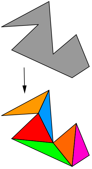
A (vertical) monotone chain is a path such that the y-coordinate never increases along the path. A simple polygon is (vertical) monotone if it is formed by two monotone chains, with the first and last vertices in common. It is possible to add some edges to a planar subdivision, in order to make all faces monotone, obtaining what is called a monotone subdivision. This process does not add any vertices to the subdivision (therefore, the size remains O(n)), and can be performed in O(n log n) time by plane sweep (it can also be performed in linear time, using polygon triangulation). Therefore, there is no loss of generality, if we restrict our data structure to the case of monotone subdivisions, as we do in this section.

The weakness of the slab decomposition is that the vertical lines create additional segments in the decomposition, making it difficult to achieve O(n) storage space. Herbert Edelsbrunner, Leonidas J. Guibas, and Jorge Stolfi discovered an optimal data structure that only uses the edges in a monotone subdivision. The idea is to use vertical monotone chains, instead of using vertical lines to partition the subdivision.^[4]

Converting this general idea to an actual efficient data structure is not a simple task. First, we need to be able to compute a monotone chain that divides the subdivision into two halves of similar sizes. Second, since some edges may be contained in several monotone chains, we need to be careful to guarantee that the storage space is O(n). Third, testing whether a point is on the left or the right side of a monotone subdivision takes O(n) time if performed naïvely.^[4]

Details on how to solve the first two issues are beyond the scope of this article. We briefly mention how to address the third issue. Using binary search, we can test whether a point is to the left or right of a monotone chain in O(log n) time. As we need to perform another nested binary search through O(log n) chains to actually determine the point location, the query time is O(log² n). To achieve O(log n) query time, we need to use fractional cascading, keeping pointers between the edges of different monotone chains.^[4]

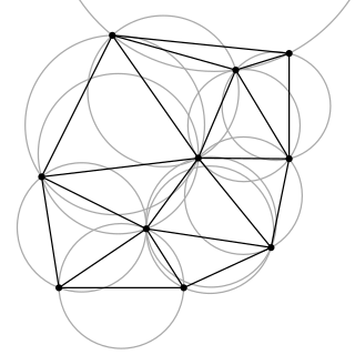
Triangulation refinement

A polygon with m vertices can be partitioned into m–2 triangles. Which can be shown by induction starting from a triangle. There are numerous algorithms to triangulate a polygon efficiently, the fastest having O(n) worst case time. Therefore, we can decompose each polygon of our subdivision in triangles, and restrict our data structure to the case of subdivisions formed exclusively by triangles. Kirkpatrick gives a data structure for point location in triangulated subdivisions with O(n) storage space and O(log n) query time.^[5]

The general idea is to build a hierarchy of triangles. To perform a query, we start by finding the top-level triangle that contains the query point. Since the number of top-level triangles is bounded by a constant, this operation can be performed in O(1) time. Each triangle has pointers to the triangles it intersects in the next level of the hierarchy, and the number of pointers is also bounded by a constant. We proceed with the query by finding which triangle contains the query point level by level.^[5]

The data structure is built in the opposite order, that is, bottom-up. We start with the triangulated subdivision, and choose an independent set of vertices to be removed. After removing the vertices, we retriangulate the subdivision. Because the subdivision is formed by triangles, a greedy algorithm can find an independent set that contains a constant fraction of the vertices. Therefore, the number of removal steps is O(log n).^[5]

Trapezoidal decomposition

A randomized approach to this problem is based on trapezoidal decomposition, or trapezoidal map. A trapezoidal decomposition is obtained by shooting vertical bullets going both up and down from each vertex in the original subdivision. The bullets stop when they hit an edge, and form a new edge in the subdivision. This way, we obtain a subset of the slab decomposition, with only O(n) edges and vertices, since for each vertex in the original subdivision we only add two new vertices and increase the number of edges by four.^[6]

A trapezoidal decomposition can be constructed by adding the segments from the original subdivision, one by one, in a random order. Initially (before no segments have been added) the trapezoidal decomposition consists of a single trapezoid, the bounding box of the subdivision. Each subsequent step uses a point location query to locate one endpoint of the next line segment, within the current trapezoidal decomposition, and then walks from the resulting trapezoid to neighboring trapezoids containing the same segment, subdividing and recombining them to form the refined decomposition. Backwards analysis, a form of analysis commonly used for this sort of randomized incremental geometry algorithm, shows that the expected number of trapezoids created for each insertion is bounded by a constant, and therefore that the total number of steps of this algorithm, outside of the point locations, is linear.^[6]

The point locations in the current subdivision, performed within this algorithm, may be done using the same structure that, at the end of the algorithm, can be used for point location queries in the final trapezoidal decomposition. This point location data structure takes the form of a directed acyclic graph, where the vertices are the trapezoids that existed at some point in the refinement, and directed edges connect each trapezoid that is no longer in the refinement to the trapezoids that replaced it. A point location query is performed by following a path in this graph, starting from the initial trapezoid, and at each step choosing the replacement trapezoid that contains the query point, until reaching a trapezoid that has not been replaced. The expected depth of a search in this digraph, starting from any query point, is O(log n). The space for the data structure is proportional to the number of trapezoids created throughout this refinement process, which in expectation is O(n).^[6]

Higher dimensions

There are no known general point location data structures with linear space and logarithmic query time for dimensions greater than 2^{[ citation needed ]}. Therefore, we need to sacrifice either query time, or storage space, or restrict ourselves to some less general type of subdivision.

In three-dimensional space, it is possible to answer point location queries in O(log² n) using O(n log n) space. The general idea is to maintain several planar point location data structures, corresponding to the intersection of the subdivision with n parallel planes that contain each subdivision vertex. A naive use of this idea would increase the storage space to O(n²). In the same fashion as in the slab decomposition, the similarity between consecutive data structures can be exploited in order to reduce the storage space to O(n log n), but the query time increases to O(log² n).^{[ citation needed ]}

In d-dimensional space, point location can be solved by recursively projecting the faces into a (d-1)-dimensional space. While the query time is O(log n), the storage space can be as high as $O(n^{2^{d}})$ . The high complexity of the d-dimensional data structures led to the study of special types of subdivision.

One important example is the case of arrangements of hyperplanes. An arrangement of n hyperplanes defines O(n^d) cells, but point location can be performed in O(log n) time with O(n^d) space by using Chazelle's hierarchical cuttings.

Another special type of subdivision is called rectilinear (or orthogonal) subdivision. In a rectilinear subdivision, all edges are parallel to one of the d orthogonal axis. In this case, point location can be answered in O(log^d-1n) time with O(n) space.

Related Research Articles

In mathematics and computational geometry, a Delaunay triangulation for a given set $P$ of discrete points in a general position is a triangulation $DT(P)$ such that no point in $P$ is inside the circumcircle of any triangle in $DT(P)$ . Delaunay triangulations maximize the minimum of all the angles of the triangles in the triangulation; they tend to avoid sliver triangles. The triangulation is named after Boris Delaunay for his work on this topic from 1934.

Computational geometry is a branch of computer science devoted to the study of algorithms which can be stated in terms of geometry. Some purely geometrical problems arise out of the study of computational geometric algorithms, and such problems are also considered to be part of computational geometry. While modern computational geometry is a recent development, it is one of the oldest fields of computing with a history stretching back to antiquity.

A quadtree is a tree data structure in which each internal node has exactly four children. Quadtrees are the two-dimensional analog of octrees and are most often used to partition a two-dimensional space by recursively subdividing it into four quadrants or regions. The data associated with a leaf cell varies by application, but the leaf cell represents a "unit of interesting spatial information".

<span class="mw-page-title-main">Polygon triangulation</span> Partition of a simple polygon into triangles

In computational geometry, polygon triangulation is the partition of a polygonal area $P$ into a set of triangles, i.e., finding a set of triangles with pairwise non-intersecting interiors whose union is $P$ .

A Euclidean minimum spanning tree of a finite set of points in the Euclidean plane or higher-dimensional Euclidean space connects the points by a system of line segments with the points as endpoints, minimizing the total length of the segments. In it, any two points can reach each other along a path through the line segments. It can be found as the minimum spanning tree of a complete graph with the points as vertices and the Euclidean distances between points as edge weights.

In geometry, a simple polygon is a polygon that does not intersect itself and has no holes. That is, it is a piecewise-linear Jordan curve consisting of finitely many line segments. These polygons include as special cases the convex polygons, star-shaped polygons, and monotone polygons.

The art gallery problem or museum problem is a well-studied visibility problem in computational geometry. It originates from the following real-world problem:

In graph theory, reachability refers to the ability to get from one vertex to another within a graph. A vertex $can reach a vertex if there exists a sequence of adjacent vertices which starts with and ends with .$

<span class="mw-page-title-main">Straight skeleton</span> Method in geometry for representing a polygon by a topological skeleton

In geometry, a straight skeleton is a method of representing a polygon by a topological skeleton. It is similar in some ways to the medial axis but differs in that the skeleton is composed of straight line segments, while the medial axis of a polygon may involve parabolic curves. However, both are homotopy-equivalent to the underlying polygon.

In computer science, fractional cascading is a technique to speed up a sequence of binary searches for the same value in a sequence of related data structures. The first binary search in the sequence takes a logarithmic amount of time, as is standard for binary searches, but successive searches in the sequence are faster. The original version of fractional cascading, introduced in two papers by Chazelle and Guibas in 1986, combined the idea of cascading, originating in range searching data structures of Lueker (1978) and Willard (1978), with the idea of fractional sampling, which originated in Chazelle (1983). Later authors introduced more complex forms of fractional cascading that allow the data structure to be maintained as the data changes by a sequence of discrete insertion and deletion events.

The dynamic convex hull problem is a class of dynamic problems in computational geometry. The problem consists in the maintenance, i.e., keeping track, of the convex hull for input data undergoing a sequence of discrete changes, i.e., when input data elements may be inserted, deleted, or modified. It should be distinguished from the kinetic convex hull, which studies similar problems for continuously moving points. Dynamic convex hull problems may be distinguished by the types of the input data and the allowed types of modification of the input data.

In computational geometry, the visibility polygon or visibility region for a point $p$ in the plane among obstacles is the possibly unbounded polygonal region of all points of the plane visible from $p$ . The visibility polygon can also be defined for visibility from a segment, or a polygon. Visibility polygons are useful in robotics, video games, and in various optimization problems such as the facility location problem and the art gallery problem.

<span class="mw-page-title-main">Monotone polygon</span>

In geometry, a polygon P in the plane is called monotone with respect to a straight line L, if every line orthogonal to L intersects the boundary of P at most twice.

<span class="mw-page-title-main">Polygonal chain</span> Connected series of line segments

In geometry, a polygonal chain is a connected series of line segments. More formally, a polygonal chain $is a curve specified by a sequence of points called its vertices. The curve itself consists of the line segments connecting the consecutive vertices.$

In graph theory, the Laman graphs are a family of sparse graphs describing the minimally rigid systems of rods and joints in the plane. Formally, a Laman graph is a graph on n vertices such that, for all k, every k-vertex subgraph has at most 2k − 3 edges, and such that the whole graph has exactly 2n − 3 edges. Laman graphs are named after Gerard Laman, of the University of Amsterdam, who in 1970 used them to characterize rigid planar structures. This characterization, however, had already been discovered in 1927 by Hilda Geiringer.

In computer science, a range tree is an ordered tree data structure to hold a list of points. It allows all points within a given range to be reported efficiently, and is typically used in two or higher dimensions. Range trees were introduced by Jon Louis Bentley in 1979. Similar data structures were discovered independently by Lueker, Lee and Wong, and Willard. The range tree is an alternative to the k-d tree. Compared to k-d trees, range trees offer faster query times of $but worse storage of, where n is the number of points stored in the tree, d is the dimension of each point and k is the number of points reported by a given query.$

In computational geometry, the Bentley–Ottmann algorithm is a sweep line algorithm for listing all crossings in a set of line segments, i.e. it finds the intersection points of line segments. It extends the Shamos–Hoey algorithm, a similar previous algorithm for testing whether or not a set of line segments has any crossings. For an input consisting of $line segments with crossings, the Bentley-Ottmann algorithm takes time . In cases where, this is an improvement on a naïve algorithm that tests every pair of segments, which takes .$

In graph theory, the planar separator theorem is a form of isoperimetric inequality for planar graphs, that states that any planar graph can be split into smaller pieces by removing a small number of vertices. Specifically, the removal of $vertices from an n -vertex graph can partition the graph into disjoint subgraphs each of which has at most vertices.$

<span class="mw-page-title-main">David Mount</span> American computer scientist

David Mount is a professor at the University of Maryland, College Park department of computer science whose research is in computational geometry.

In geometry, a partition of a polygon is a set of primitive units, which do not overlap and whose union equals the polygon. A polygon partition problem is a problem of finding a partition which is minimal in some sense, for example a partition with a smallest number of units or with units of smallest total side-length.

References

Notes

↑ Bern 1990.
1 2 Dobkin & Lipton 1976.
↑ Sarnak & Tarjan 1986.
1 2 3 Edelsbrunner, Guibas & Stolfi 1986.
1 2 3 Kirkpatrick 1983.
1 2 3 de Berg et al. 2000.

Sources

de Berg, Mark; van Kreveld, Marc; Overmars, Mark; Schwarzkopf, Otfried (2000). "Chapter 6: Point location". Computational Geometry (2nd revised ed.). Springer-Verlag. pp. 121–146. ISBN 3-540-65620-0.
Bern, Marshall (1990). "Hidden surface removal for rectangles". Journal of Computer and System Sciences. 40 (1): 49–69. doi: 10.1016/0022-0000(90)90018-G . MR 1047289.
Dobkin, David; Lipton, Richard J. (1976). "Multidimensional searching problems". SIAM Journal on Computing . 5 (2): 181–186. doi:10.1137/0205015.
Edelsbrunner, Herbert; Guibas, Leonidas J.; Stolfi, Jorge (1986). "Optimal point location in a monotone subdivision". SIAM Journal on Computing . 15 (2): 317–340. doi:10.1137/0215023.
Kirkpatrick, David G. (1983). "Optimal search in planar subdivisions". SIAM Journal on Computing . 12 (1): 28–35. CiteSeerX 10.1.1.461.1866 . doi:10.1137/0212002.
Sarnak, Neil; Tarjan, Robert E. (1986). "Planar point location using persistent search trees". Communications of the ACM . 29 (7): 669–679. doi:10.1145/6138.6151.

External links

Point-Location Source Repository at Stony Brook University
Point-Location Queries in CGAL, the Computational Geometry Algorithms Library

This page is based on this Wikipedia article
Text is available under the CC BY-SA 4.0 license; additional terms may apply.
Images, videos and audio are available under their respective licenses.

[FOOTNOTEBern1990-1] Bern 1990.

[FOOTNOTEDobkinLipton1976-2] 1 2 Dobkin & Lipton 1976.

[FOOTNOTESarnakTarjan1986-3] Sarnak & Tarjan 1986.

[FOOTNOTEEdelsbrunnerGuibasStolfi1986-4] 1 2 3 Edelsbrunner, Guibas & Stolfi 1986.

[FOOTNOTEKirkpatrick1983-5] 1 2 3 Kirkpatrick 1983.

[FOOTNOTEde_Bergvan_KreveldOvermarsSchwarzkopf2000-6] 1 2 3 de Berg et al. 2000.

[1]

[2]

[3]

[4]

[5]

[6]