In probability theory and statistics, kurtosis refers to the degree of “tailedness” in the probability distribution of a real-valued random variable. Similar to skewness, kurtosis provides insight into specific characteristics of a distribution. Various methods exist for quantifying kurtosis in theoretical distributions, and corresponding techniques allow estimation based on sample data from a population. It’s important to note that different measures of kurtosis can yield varying interpretations.
In mathematics, Pascal's triangle is an infinite triangular array of the binomial coefficients which play a crucial role in probability theory, combinatorics, and algebra. In much of the Western world, it is named after the French mathematician Blaise Pascal, although other mathematicians studied it centuries before him in Persia, India, China, Germany, and Italy.

In probability theory and statistics, the multivariate normal distribution, multivariate Gaussian distribution, or joint normal distribution is a generalization of the one-dimensional (univariate) normal distribution to higher dimensions. One definition is that a random vector is said to be k-variate normally distributed if every linear combination of its k components has a univariate normal distribution. Its importance derives mainly from the multivariate central limit theorem. The multivariate normal distribution is often used to describe, at least approximately, any set of (possibly) correlated real-valued random variables, each of which clusters around a mean value.

In statistics, correlation or dependence is any statistical relationship, whether causal or not, between two random variables or bivariate data. Although in the broadest sense, "correlation" may indicate any type of association, in statistics it usually refers to the degree to which a pair of variables are linearly related. Familiar examples of dependent phenomena include the correlation between the height of parents and their offspring, and the correlation between the price of a good and the quantity the consumers are willing to purchase, as it is depicted in the so-called demand curve.
In vector calculus, the Jacobian matrix of a vector-valued function of several variables is the matrix of all its first-order partial derivatives. When this matrix is square, that is, when the function takes the same number of variables as input as the number of vector components of its output, its determinant is referred to as the Jacobian determinant. Both the matrix and the determinant are often referred to simply as the Jacobian in literature. They are named after Carl Gustav Jacob Jacobi.
In mathematics, the falling factorial is defined as the polynomial
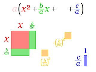
In elementary algebra, completing the square is a technique for converting a quadratic polynomial of the form to the form for some values of h and k.
In numerical analysis, one of the most important problems is designing efficient and stable algorithms for finding the eigenvalues of a matrix. These eigenvalue algorithms may also find eigenvectors.
In physics, the S-matrix or scattering matrix relates the initial state and the final state of a physical system undergoing a scattering process. It is used in quantum mechanics, scattering theory and quantum field theory (QFT).
In mathematics, the kernel of a linear map, also known as the null space or nullspace, is the part of the domain which is mapped to the zero vector of the co-domain; the kernel is always a linear subspace of the domain. That is, given a linear map L : V → W between two vector spaces V and W, the kernel of L is the vector space of all elements v of V such that L(v) = 0, where 0 denotes the zero vector in W, or more symbolically:
In probability theory and statistics, the generalized extreme value (GEV) distribution is a family of continuous probability distributions developed within extreme value theory to combine the Gumbel, Fréchet and Weibull families also known as type I, II and III extreme value distributions. By the extreme value theorem the GEV distribution is the only possible limit distribution of properly normalized maxima of a sequence of independent and identically distributed random variables. that a limit distribution needs to exist, which requires regularity conditions on the tail of the distribution. Despite this, the GEV distribution is often used as an approximation to model the maxima of long (finite) sequences of random variables.

A transversely isotropic material is one with physical properties that are symmetric about an axis that is normal to a plane of isotropy. This transverse plane has infinite planes of symmetry and thus, within this plane, the material properties are the same in all directions. Hence, such materials are also known as "polar anisotropic" materials. In geophysics, vertically transverse isotropy (VTI) is also known as radial anisotropy.
In linear algebra, an eigenvector or characteristic vector is a vector that has its direction unchanged by a given linear transformation. More precisely, an eigenvector, , of a linear transformation, , is scaled by a constant factor, , when the linear transformation is applied to it: . It is often important to know these vectors in linear algebra. The corresponding eigenvalue, characteristic value, or characteristic root is the multiplying factor .

In material science and solid mechanics, orthotropic materials have material properties at a particular point which differ along three orthogonal axes, where each axis has twofold rotational symmetry. These directional differences in strength can be quantified with Hankinson's equation.
The Wigner D-matrix is a unitary matrix in an irreducible representation of the groups SU(2) and SO(3). It was introduced in 1927 by Eugene Wigner, and plays a fundamental role in the quantum mechanical theory of angular momentum. The complex conjugate of the D-matrix is an eigenfunction of the Hamiltonian of spherical and symmetric rigid rotors. The letter D stands for Darstellung, which means "representation" in German.
The sample mean or empirical mean, and the sample covariance or empirical covariance are statistics computed from a sample of data on one or more random variables.

In probability and statistics, the quantile function outputs the value of a random variable such that its probability is less than or equal to an input probability value. Intuitively, the quantile function associates with a range at and below a probability input the likelihood that a random variable is realized in that range for some probability distribution. It is also called the percentile function, percent-point function, inverse cumulative distribution function or inverse distribution function.

In mathematics, a matrix is a rectangular array or table of numbers, symbols, or expressions, with elements or entries arranged in rows and columns, which is used to represent a mathematical object or property of such an object.
The purpose of this page is to provide supplementary materials for the ordinary least squares article, reducing the load of the main article with mathematics and improving its accessibility, while at the same time retaining the completeness of exposition.
Linear least squares (LLS) is the least squares approximation of linear functions to data. It is a set of formulations for solving statistical problems involved in linear regression, including variants for ordinary (unweighted), weighted, and generalized (correlated) residuals. Numerical methods for linear least squares include inverting the matrix of the normal equations and orthogonal decomposition methods.


