A quantum limit in physics is a limit on measurement accuracy at quantum scales.[1] Depending on the context, the limit may be absolute (such as the Heisenberg limit), or it may only apply when the experiment is conducted with naturally occurring quantum states (e.g. the standard quantum limit in interferometry) and can be circumvented with advanced state preparation and measurement schemes.
The usage of the term standard quantum limit or SQL is, however, broader than just interferometry. In principle, any linear measurement of a quantum mechanical observable of a system under study that does not commute with itself at different times leads to such limits. In short, it is the Heisenberg uncertainty principle that is the cause.
A schematic description of how physical measurement process is described in quantum mechanics
A more detailed explanation would be that any measurement in quantum mechanics involves at least two parties, an Object and a Meter. The former is the system whose observable, say , we want to measure. The latter is the system we couple to the Object in order to infer the value of of the Object by recording some chosen observable, , of this system, e.g. the position of the pointer on a scale of the Meter. This, in a nutshell, is a model of most of the measurements happening in physics, known as indirect measurements (see pp.38–42 of [1]). So any measurement is a result of interaction and that acts in both ways. Therefore, the Meter acts on the Object during each measurement, usually via the quantity, , conjugate to the readout observable , thus perturbing the value of measured observable and modifying the results of subsequent measurements. This is known as back action (quantum) of the Meter on the system under measurement.
At the same time, quantum mechanics prescribes that readout observable of the Meter should have an inherent uncertainty, , additive to and independent of the value of the measured quantity . This one is known as measurement imprecision or measurement noise. Because of the Heisenberg uncertainty principle, this imprecision cannot be arbitrary and is linked to the back-action perturbation by the uncertainty relation:
where is a standard deviation of observable and stands for expectation value of in whatever quantum state the system is. The equality is reached if the system is in a minimum uncertainty state. The consequence for our case is that the more precise is our measurement, i.e the smaller is , the larger will be perturbation the Meter exerts on the measured observable . Therefore, the readout of the meter will, in general, consist of three terms:
where is a value of that the Object would have, were it not coupled to the Meter, and is the perturbation to the value of caused by back action force, . The uncertainty of the latter is proportional to . Thus, there is a minimal value, or the limit to the precision one can get in such a measurement, provided that and are uncorrelated.[2][3]
The terms "quantum limit" and "standard quantum limit" are sometimes used interchangeably. Usually, "quantum limit" is a general term which refers to any restriction on measurement due to quantum effects, while the "standard quantum limit" in any given context refers to a quantum limit which is ubiquitous in that context.
Examples
Displacement measurement
Consider a very simple measurement scheme, which, nevertheless, embodies all key features of a general position measurement. In the scheme shown in Figure, a sequence of very short light pulses are used to monitor the displacement of a probe body . The position of is probed periodically with time interval . We assume mass large enough to neglect the displacement inflicted by the pulses regular (classical) radiation pressure in the course of measurement process.
Simplified scheme of optical measurement of mechanical object position
Then each -th pulse, when reflected, carries a phase shift proportional to the value of the test-mass position at the moment of reflection:
(1)
where , is the light frequency, is the pulse number and is the initial (random) phase of the -th pulse. We assume that the mean value of all these phases is equal to zero, , and their root mean square (RMS) uncertainty is equal to .
The reflected pulses are detected by a phase-sensitive device (the phase detector). The implementation of an optical phase detector can be done using, e.g.homodyne or heterodyne detection scheme (see Section 2.3 in [2] and references therein), or other such read-out techniques.
In this example, light pulse phase serves as the readout observable of the Meter. Then we suppose that the phase measurement error introduced by the detector is much smaller than the initial uncertainty of the phases . In this case, the initial uncertainty will be the only source of the position measurement error:
(2)
For convenience, we renormalise Eq. (1) as the equivalent test-mass displacement:
(3)
where
are the independent random values with the RMS uncertainties given by Eq. (2).
Upon reflection, each light pulse kicks the test mass, transferring to it a back-action momentum equal to
(4)
where and are the test-mass momentum values just before and just after the light pulse reflection, and is the energy of the -th pulse, that plays the role of back action observable of the Meter. The major part of this perturbation is contributed by classical radiation pressure:
with the mean energy of the pulses. Therefore, one could neglect its effect, for it could be either subtracted from the measurement result or compensated by an actuator. The random part, which cannot be compensated, is proportional to the deviation of the pulse energy:
and its RMS uncertainly is equal to
(5)
with the RMS uncertainty of the pulse energy.
Assuming the mirror is free (which is a fair approximation if time interval between pulses is much shorter than the period of suspended mirror oscillations, ), one can estimate an additional displacement caused by the back action of the -th pulse that will contribute to the uncertainty of the subsequent measurement by the pulse time later:
Its uncertainty will be simply
If we now want to estimate how much has the mirror moved between the and pulses, i.e. its displacement, we will have to deal with three additional uncertainties that limit precision of our estimate:
where we assumed all contributions to our measurement uncertainty statistically independent and thus got sum uncertainty by summation of standard deviations. If we further assume that all light pulses are similar and have the same phase uncertainty, thence .
Now, what is the minimum this sum and what is the minimum error one can get in this simple estimate? The answer ensues from quantum mechanics, if we recall that energy and the phase of each pulse are canonically conjugate observables and thus obey the following uncertainty relation:
Therefore, it follows from Eqs. (2 and 5) that the position measurement error and the momentum perturbation due to back action also satisfy the uncertainty relation:
Taking this relation into account, the minimal uncertainty, , the light pulse should have in order not to perturb the mirror too much, should be equal to yielding for both . Thus the minimal displacement measurement error that is prescribed by quantum mechanics read:
This is the Standard Quantum Limit for such a 2-pulse procedure. In principle, if we limit our measurement to two pulses only and do not care about perturbing mirror position afterwards, the second pulse measurement uncertainty, , can, in theory, be reduced to 0 (it will yield, of course, ) and the limit of displacement measurement error will reduce to:
which is known as the Standard Quantum Limit for the measurement of free mass displacement.
This example represents a simple particular case of a linear measurement. This class of measurement schemes can be fully described by two linear equations of the form~(3) and (4), provided that both the measurement uncertainty and the object back-action perturbation ( and in this case) are statistically independent of the test object initial quantum state and satisfy the same uncertainty relation as the measured observable and its canonically conjugate counterpart (the object position and momentum in this case).
Usage in quantum optics
In the context of interferometry or other optical measurements, the standard quantum limit usually refers to the minimum level of quantum noise which is obtainable without squeezed states.[4]
There is additionally a quantum limit for phase noise, reachable only by a laser at high noise frequencies.
In spectroscopy, the shortest wavelength in an X-ray spectrum is called the quantum limit.[5]
Misleading relation to the classical limit
Note that due to an overloading of the word "limit", the classical limit is not the opposite of the quantum limit. In "quantum limit", "limit" is being used in the sense of a physical limitation (e.g. the Armstrong limit). In "classical limit", "limit" is used in the sense of a limiting process. (Note that there is no simple rigorous mathematical limit which fully recovers classical mechanics from quantum mechanics, the Ehrenfest theorem notwithstanding. Nevertheless, in the phase space formulation of quantum mechanics, such limits are more systematic and practical.)
In quantum mechanics, the uncertainty principle is any of a variety of mathematical inequalities asserting a fundamental limit to the accuracy with which the values for certain pairs of physical quantities of a particle, such as position, x, and momentum, p, can be predicted from initial conditions.
In quantum physics, a quantum fluctuation is the temporary random change in the amount of energy in a point in space, as prescribed by Werner Heisenberg's uncertainty principle. They are minute random fluctuations in the values of the fields which represent elementary particles, such as electric and magnetic fields which represent the electromagnetic force carried by photons, W and Z fields which carry the weak force, and gluon fields which carry the strong force. Vacuum fluctuations appear as virtual particles, which are always created in particle-antiparticle pairs. Since they are created spontaneously without a source of energy, vacuum fluctuations and virtual particles are said to violate the conservation of energy. This is theoretically allowable because the particles annihilate each other within a time limit determined by the uncertainty principle so they are not directly observable. The uncertainty principle states the uncertainty in energy and time can be related by , where 1/2ħ ≈ 5.27286×10⁻³⁵ Js. This means that pairs of virtual particles with energy and lifetime shorter than are continually created and annihilated in empty space. Although the particles are not directly detectable, the cumulative effects of these particles are measurable. For example, without quantum fluctuations, the "bare" mass and charge of elementary particles would be infinite; from renormalization theory the shielding effect of the cloud of virtual particles is responsible for the finite mass and charge of elementary particles. Another consequence is the Casimir effect. One of the first observations which was evidence for vacuum fluctuations was the Lamb shift in hydrogen. In July 2020, scientists reported that quantum vacuum fluctuations can influence the motion of macroscopic, human-scale objects by measuring correlations below the standard quantum limit between the position/momentum uncertainty of the mirrors of LIGO and the photon number/phase uncertainty of light that they reflect.
In physics, an operator is a function over a space of physical states onto another space of physical states. The simplest example of the utility of operators is the study of symmetry. Because of this, they are very useful tools in classical mechanics. Operators are even more important in quantum mechanics, where they form an intrinsic part of the formulation of the theory.
The path integral formulation is a description in quantum mechanics that generalizes the action principle of classical mechanics. It replaces the classical notion of a single, unique classical trajectory for a system with a sum, or functional integral, over an infinity of quantum-mechanically possible trajectories to compute a quantum amplitude.
In physics, a squeezed coherent state is a quantum state that is usually described by two non-commuting observables having continuous spectra of eigenvalues. Examples are position and momentum of a particle, and the (dimension-less) electric field in the amplitude and in the mode of a light wave. The product of the standard deviations of two such operators obeys the uncertainty principle:
In quantum mechanics, the canonical commutation relation is the fundamental relation between canonical conjugate quantities. For example,
In quantum information theory, a quantum channel is a communication channel which can transmit quantum information, as well as classical information. An example of quantum information is the state of a qubit. An example of classical information is a text document transmitted over the Internet.
In quantum field theory, the quantum effective action is a modified expression for the classical action taking into account quantum corrections while ensuring that the principle of least action applies, meaning that extremizing the effective action yields the equations of motion for the vacuum expectation values of the quantum fields. The effective action also acts as a generating functional for one-particle irreducible correlation functions. The potential component of the effective action is called the effective potential, with the expectation value of the true vacuum being the minimum of this potential rather than the classical potential, making it important for studying spontaneous symmetry breaking.
In physics, a sigma model is a field theory that describes the field as a point particle confined to move on a fixed manifold. This manifold can be taken to be any Riemannian manifold, although it is most commonly taken to be either a Lie group or a symmetric space. The model may or may not be quantized. An example of the non-quantized version is the Skyrme model; it cannot be quantized due to non-linearities of power greater than 4. In general, sigma models admit (classical) topological soliton solutions, for example, the Skyrmion for the Skyrme model. When the sigma field is coupled to a gauge field, the resulting model is described by Ginzburg–Landau theory. This article is primarily devoted to the classical field theory of the sigma model; the corresponding quantized theory is presented in the article titled "non-linear sigma model".
Quantum noise is noise arising from the indeterminate state of matter in accordance with fundamental principles of quantum mechanics, specifically the uncertainty principle and via zero-point energy fluctuations. Quantum noise is due to the apparently discrete nature of the small quantum constituents such as electrons, as well as the discrete nature of quantum effects, such as photocurrents.
In theoretical physics, background field method is a useful procedure to calculate the effective action of a quantum field theory by expanding a quantum field around a classical "background" value B:
In quantum mechanics, the position operator is the operator that corresponds to the position observable of a particle.
In theoretical physics, scalar field theory can refer to a relativistically invariant classical or quantum theory of scalar fields. A scalar field is invariant under any Lorentz transformation.
In physics, a quantum vortex represents a quantized flux circulation of some physical quantity. In most cases, quantum vortices are a type of topological defect exhibited in superfluids and superconductors. The existence of quantum vortices was first predicted by Lars Onsager in 1949 in connection with superfluid helium. Onsager reasoned that quantisation of vorticity is a direct consequence of the existence of a superfluid order parameter as a spatially continuous wavefunction. Onsager also pointed out that quantum vortices describe the circulation of superfluid and conjectured that their excitations are responsible for superfluid phase transitions. These ideas of Onsager were further developed by Richard Feynman in 1955 and in 1957 were applied to describe the magnetic phase diagram of type-II superconductors by Alexei Alexeyevich Abrikosov. In 1935 Fritz London published a very closely related work on magnetic flux quantization in superconductors. London's fluxoid can also be viewed as a quantum vortex.
Wick's theorem is a method of reducing high-order derivatives to a combinatorics problem. It is named after Italian physicist Gian-Carlo Wick. It is used extensively in quantum field theory to reduce arbitrary products of creation and annihilation operators to sums of products of pairs of these operators. This allows for the use of Green's function methods, and consequently the use of Feynman diagrams in the field under study. A more general idea in probability theory is Isserlis' theorem.
Lagrangian field theory is a formalism in classical field theory. It is the field-theoretic analogue of Lagrangian mechanics. Lagrangian mechanics is used to analyze the motion of a system of discrete particles each with a finite number of degrees of freedom. Lagrangian field theory applies to continua and fields, which have an infinite number of degrees of freedom.
In theoretical physics, Hamiltonian field theory is the field-theoretic analogue to classical Hamiltonian mechanics. It is a formalism in classical field theory alongside Lagrangian field theory. It also has applications in quantum field theory.
Lightfieldmicroscopy (LFM) is a scanning-free 3-dimensional (3D) microscopic imaging method based on the theory of light field. This technique allows sub-second (~10 Hz) large volumetric imaging with ~1 μm spatial resolution in the condition of weak scattering and semi-transparence, which has never been achieved by other methods. Just as in traditional light field rendering, there are two steps for LFM imaging: light field capture and processing. In most setups, a microlens array is used to capture the light field. As for processing, it can be based on two kinds of representations of light propagation: the ray optics picture and the wave optics picture. The Stanford University Computer Graphics Laboratory published their first prototype LFM in 2006 and has been working on the cutting edge since then.
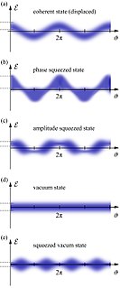
In quantum physics, light is in a squeezed state if its electric field strength Ԑ for some phases has a quantum uncertainty smaller than that of a coherent state. The term squeezing thus refers to a reduced quantum uncertainty. To obey Heisenberg's uncertainty relation, a squeezed state must also have phases at which the electric field uncertainty is anti-squeezed, i.e. larger than that of a coherent state. Since 2019, the gravitational-wave observatories LIGO and Virgo employ squeezed laser light, which has significantly increased the rate of observed gravitational-wave events.
In theoretical physics, more specifically in quantum field theory and supersymmetry, supersymmetric Yang–Mills, also known as super Yang–Mills and abbreviated to SYM, is a supersymmetric generalization of Yang–Mills theory, which is a gauge theory that plays an important part in the mathematical formulation of forces in particle physics.
This page is based on this Wikipedia article Text is available under the CC BY-SA 4.0 license; additional terms may apply. Images, videos and audio are available under their respective licenses.