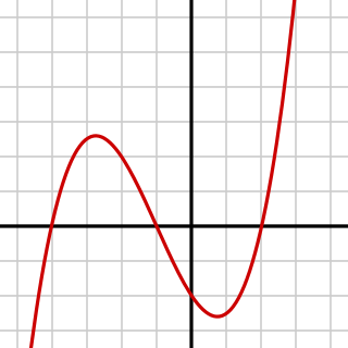
Graph of a polynomial function of degree 4, with its 4 roots and 3 critical points.
where a≠0.
The quartic is the highest order polynomial equation that can be solved by radicals in the general case (i.e., one in which the coefficients can take any value).
History
Lodovico Ferrari is attributed with the discovery of the solution to the quartic in 1540, but since this solution, like all algebraic solutions of the quartic, requires the solution of a cubic to be found, it could not be published immediately.[1] The solution of the quartic was published together with that of the cubic by Ferrari's mentor Gerolamo Cardano in the book Ars Magna (1545).
The proof that this was the highest order general polynomial for which such solutions could be found was first given in the Abel–Ruffini theorem in 1824, proving that all attempts at solving the higher order polynomials would be futile. The notes left by Évariste Galois before his death in a duel in 1832 later led to an elegant complete theory of the roots of polynomials, of which this theorem was one result.[2]
Solving a quartic equation, special cases
Consider a quartic equation expressed in the form :
There exists a general formula for finding the roots to quartic equations, provided the coefficient of the leading term is non-zero. However, since the general method is quite complex and susceptible to errors in execution, it is better to apply one of the special cases listed below if possible.
If the constant term a4=0, then one of the roots is x=0, and the other roots can be found by dividing by x, and solving the resulting cubic equation,
Evident roots: 1 and −1 and −k
Call our quartic polynomial Q(x). Since 1 raised to any power is 1,
Thus if Q(1) = 0 and so x = 1 is a root of Q(x). It can similarly be shown that if x = −1 is a root.
In either case the full quartic can then be divided by the factor (x − 1) or (x + 1) respectively yielding a new cubic polynomial, which can be solved to find the quartic's other roots.
If and then is a root of the equation. The full quartic can then be factorized this way:
Alternatively, if and then x = 0 and x = −k become two known roots. Q(x) divided by x(x + k) is a quadratic polynomial.
Biquadratic equations
A quartic equation where a3 and a1 are equal to 0 takes the form
and thus is a biquadratic equation, which is easy to solve: let , so our equation turns to
which is a simple quadratic equation, whose solutions are easily found using the quadratic formula:
When we've solved it (i.e. found these two z values), we can extract x from them
If either of the z solutions were negative or complex numbers, then some of the x solutions are complex numbers.
Quasi-symmetric equations
Steps:
Divide by x2.
Use variable change z = x + m/x.
So, z2 = x2 + (m/x)2 + 2m.
This leads to:
,
,
(a quadratic in z = x + m/x)
Multiple roots
If the quartic has a double root, it can be found by taking the polynomial greatest common divisor with its derivative. Then they can be divided out and the resulting quadratic equation solved.
In general, there exist only four possible cases of quartic equations with multiple roots, which are listed below:[3]
Multiplicity-4 (M4): when the general quartic equation can be expressed as , for some real number. This case can always be reduced to a biquadratic equation.
Multiplicity-3 (M3): when the general quartic equation can be expressed as , where and are a couple of two different real numbers. This is the only case that can never be reduced to a biquadratic equation.
Double Multiplicity-2 (DM2): when the general quartic equation can be expressed as , where and are a couple of two different real numbers or a couple of non-real complex conjugate numbers. This case can also always be reduced to a biquadratic equation.
Single Multiplicity-2 (SM2): when the general quartic equation can be expressed as , where , , and are three different real numbers or is a real number and and are a couple of non-real complex conjugate numbers. This case is divided into two subcases, those that can be reduced to a biquadratic equation and those in which this is impossible.
So, if the three non-monic coefficients of the depressed quartic equation, , in terms of the five coefficients of the general quartic equation are given as follows: , and , then the criteria to identify a priori each case of quartic equations with multiple roots and their respective solutions are exposed below.
M4. The general quartic equation corresponds to this case whenever , so the four roots of this equation are given as follows: .
M3. The general quartic equation corresponds to this case whenever and , so the four roots of this equation are given as follows: and , whether ; otherwise, and .
DM2. The general quartic equation corresponds to this case whenever , so the four roots of this equation are given as follows: and .
Biquadratic SM2. The general quartic equation corresponds to this subcase of the SM2 equations whenever , so the four roots of this equation are given as follows: , and .
Non-Biquadratic SM2. The general quartic equation corresponds to this subcase of the SM2 equations whenever , so the four roots of this equation are given by the following formula:[4], where , and .
The general case
The quartic formula.
To begin, the quartic must first be converted to a depressed quartic.
Converting to a depressed quartic
Let
(1')
be the general quartic equation which it is desired to solve. Divide both sides by A,
The first step, if B is not already zero, should be to eliminate the x3 term. To do this, change variables from x to u, such that
Then
Expanding the powers of the binomials produces
Collecting the same powers of u yields
Now rename the coefficients of u. Let
The resulting equation is
(1)
which is a depressed quartic equation.
If then we have the special case of a biquadratic equation, which is easily solved, as explained above. Note that the general solution, given below, will not work for the special case The equation must be solved as a biquadratic.
In either case, once the depressed quartic is solved for u, substituting those values into
produces the values for x that solve the original quartic.
Solving a depressed quartic when b ≠ 0
After converting to a depressed quartic equation
and excluding the special case b = 0, which is solved as a biquadratic, we assume from here on that b ≠ 0 .
We will separate the terms left and right as
and add in terms to both sides which make them both into perfect squares.
Subtracting, we get the difference of two squares which is the product of the sum and difference of their roots
which can be solved by applying the quadratic formula to each of the two factors. So the possible values of u are:
or
Using another y from among the three roots of the cubic simply causes these same four values of u to appear in a different order. The solutions of the cubic are:
using any one of the three possible cube roots. A wise strategy is to choose the sign of the square-root that makes the absolute value of w as large as possible.
Ferrari's solution
Otherwise, the depressed quartic can be solved by means of a method discovered by Lodovico Ferrari. Once the depressed quartic has been obtained, the next step is to add the valid identity
The effect has been to fold up the u4 term into a perfect square: (u2+a)2. The second term, au2 did not disappear, but its sign has changed and it has been moved to the right side.
The next step is to insert a variable y into the perfect square on the left side of equation (2), and a corresponding 2y into the coefficient of u2 in the right side. To accomplish these insertions, the following valid formulas will be added to equation (2),
The objective now is to choose a value for y such that the right side of equation (3) becomes a perfect square. This can be done by letting the discriminant of the quadratic function become zero. To explain this, first expand a perfect square so that it equals a quadratic function:
The quadratic function on the right side has three coefficients. It can be verified that squaring the second coefficient and then subtracting four times the product of the first and third coefficients yields zero:
Therefore to make the right side of equation (3) into a perfect square, the following equation must be solved:
Multiply the binomial with the polynomial,
Divide both sides by −4, and move the −b2/4 to the right,
Divide both sides by 2,
(4)
This is a cubic equation in y. Solve for y using any method for solving such equations (e.g. conversion to a reduced cubic and application of Cardano's formula). Any of the three possible roots will do.
Folding the second perfect square
With the value for y so selected, it is now known that the right side of equation (3) is a perfect square of the form
(This is correct for both signs of square root, as long as the same sign is taken for both square roots. A ± is redundant, as it would be absorbed by another ± a few equations further down this page.)
so that it can be folded:
Note: If b ≠ 0 then a + 2y ≠ 0. If b = 0 then this would be a biquadratic equation, which we solved earlier.
This is the solution of the depressed quartic, therefore the solutions of the original quartic equation are
(6')
Remember: The two come from the same place in equation (5'), and should both have the same sign, while the sign of is independent.
Summary of Ferrari's method
Given the quartic equation
its solution can be found by means of the following calculations:
If then
Otherwise, continue with
(either sign of the square root will do)
(there are 3 complex roots, any one of them will do)
The two ±s must have the same sign, the ±t is independent. To get all roots, compute x for ±s,±t = +,+ and for +,−; and for −,+ and for −,−. This formula handles repeated roots without problem.
Ferrari was the first to discover one of these labyrinthine solutions[citation needed]. The equation which he solved was
which was already in depressed form. It has a pair of solutions which can be found with the set of formulas shown above.
Ferrari's solution in the special case of real coefficients
If the coefficients of the quartic equation are real then the nested depressed cubic equation (5) also has real coefficients, thus it has at least one real root.
This means that (5) has a real root greater than , and therefore that (4) has a real root greater than .
Using this root the term in (8) is always real, which ensures that the two quadratic equations (8) have real coefficients.[5]
Obtaining alternative solutions the hard way
It could happen that one only obtained one solution through the formulae above, because not all four sign patterns are tried for four solutions, and the solution obtained is complex. It may also be the case that one is only looking for a real solution. Let x1 denote the complex solution. If all the original coefficients A, B, C, D and E are real—which should be the case when one desires only real solutions – then there is another complex solution x2 which is the complex conjugate of x1. If the other two roots are denoted as x3 and x4 then the quartic equation can be expressed as
but this quartic equation is equivalent to the product of two quadratic equations:
One of these two solutions should be the desired real solution.
Alternative methods
Quick and memorable solution from first principles
Most textbook solutions of the quartic equation require a substitution that is hard to memorize. Here is an approach that makes it easy to understand. The job is done if we can factor the quartic equation into a product of two quadratics. Let
By equating coefficients, this results in the following set of simultaneous equations:
This is harder to solve than it looks, but if we start again with a depressed quartic where , which can be obtained by substituting for , then , and:
It's now easy to eliminate both and by doing the following:
If we set , then this equation turns into the cubic equation:
which is solved elsewhere. Once you have , then:
The symmetries in this solution are easy to see. There are three roots of the cubic, corresponding to the three ways that a quartic can be factored into two quadratics, and choosing positive or negative values of for the square root of merely exchanges the two quadratics with one another.
Galois theory and factorization
The symmetric groupS4 on four elements has the Klein four-group as a normal subgroup. This suggests using a resolvent whose roots may be variously described as a discrete Fourier transform or a Hadamard matrix transform of the roots. Suppose ri for i from 0 to 3 are roots of
If we now set
then since the transformation is an involution, we may express the roots in terms of the four si in exactly the same way. Since we know the value s0 = −b/2, we really only need the values for s1, s2 and s3. These we may find by expanding the polynomial
which if we make the simplifying assumption that b=0, is equal to
This polynomial is of degree six, but only of degree three in z2, and so the corresponding equation is solvable. By trial we can determine which three roots are the correct ones, and hence find the solutions of the quartic.
We can remove any requirement for trial by using a root of the same resolvent polynomial for factoring; if w is any root of (3), and if
then
We therefore can solve the quartic by solving for w and then solving for the roots of the two factors using the quadratic formula.
Approximate methods
The methods described above are, in principle, exact root-finding methods. It is also possible to use successive approximation methods which iteratively converge towards the roots, such as the Durand–Kerner method. Iterative methods are the only ones available for quintic and higher-order equations, beyond trivial or special cases.
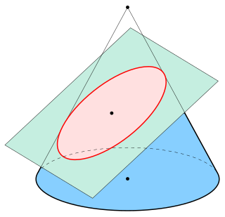
In mathematics, an ellipse is a plane curve surrounding two focal points, such that for all points on the curve, the sum of the two distances to the focal points is a constant. It generalizes a circle, which is the special type of ellipse in which the two focal points are the same. The elongation of an ellipse is measured by its eccentricity , a number ranging from to .
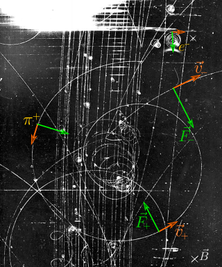
In physics, specifically in electromagnetism, the Lorentz force is the combination of electric and magnetic force on a point charge due to electromagnetic fields. A particle of charge q moving with a velocity v in an electric field E and a magnetic field B experiences a force of
In mathematics, a quadratic equation is an equation that can be rearranged in standard form as
In elementary algebra, the quadratic formula is a closed-form expression describing the solutions of a quadratic equation. Other ways of solving quadratic equations, such as completing the square, yield the same solutions.
In mathematics and physics, the heat equation is a certain partial differential equation. Solutions of the heat equation are sometimes known as caloric functions. The theory of the heat equation was first developed by Joseph Fourier in 1822 for the purpose of modeling how a quantity such as heat diffuses through a given region.
In algebra, a cubic equation in one variable is an equation of the form
In mathematics, a quintic function is a function of the form
In algebra, a quartic function is a function of the form
In geodesy, conversion among different geographic coordinate systems is made necessary by the different geographic coordinate systems in use across the world and over time. Coordinate conversion is composed of a number of different types of conversion: format change of geographic coordinates, conversion of coordinate systems, or transformation to different geodetic datums. Geographic coordinate conversion has applications in cartography, surveying, navigation and geographic information systems.
In mathematics, the Jacobi elliptic functions are a set of basic elliptic functions. They are found in the description of the motion of a pendulum, as well as in the design of electronic elliptic filters. While trigonometric functions are defined with reference to a circle, the Jacobi elliptic functions are a generalization which refer to other conic sections, the ellipse in particular. The relation to trigonometric functions is contained in the notation, for example, by the matching notation for . The Jacobi elliptic functions are used more often in practical problems than the Weierstrass elliptic functions as they do not require notions of complex analysis to be defined and/or understood. They were introduced by Carl Gustav Jakob Jacobi. Carl Friedrich Gauss had already studied special Jacobi elliptic functions in 1797, the lemniscate elliptic functions in particular, but his work was published much later.
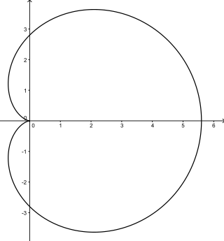
In geometry, a cardioid is a plane curve traced by a point on the perimeter of a circle that is rolling around a fixed circle of the same radius. It can also be defined as an epicycloid having a single cusp. It is also a type of sinusoidal spiral, and an inverse curve of the parabola with the focus as the center of inversion. A cardioid can also be defined as the set of points of reflections of a fixed point on a circle through all tangents to the circle.
In mathematics, the matrix exponential is a matrix function on square matrices analogous to the ordinary exponential function. It is used to solve systems of linear differential equations. In the theory of Lie groups, the matrix exponential gives the exponential map between a matrix Lie algebra and the corresponding Lie group.
In the mathematical field of complex analysis, contour integration is a method of evaluating certain integrals along paths in the complex plane.
In algebra, a nested radical is a radical expression that contains (nests) another radical expression. Examples include
In algebra, the Bring radical or ultraradical of a real number a is the unique real root of the polynomial
In mathematics, the lemniscate elliptic functions are elliptic functions related to the arc length of the lemniscate of Bernoulli. They were first studied by Giulio Fagnano in 1718 and later by Leonhard Euler and Carl Friedrich Gauss, among others.
In geometry, the trilinear coordinatesx : y : z of a point relative to a given triangle describe the relative directed distances from the three sidelines of the triangle. Trilinear coordinates are an example of homogeneous coordinates. The ratio x : y is the ratio of the perpendicular distances from the point to the sides opposite vertices A and B respectively; the ratio y : z is the ratio of the perpendicular distances from the point to the sidelines opposite vertices B and C respectively; and likewise for z : x and vertices C and A.
In mathematics, the Jacobi curve is a representation of an elliptic curve different from the usual one defined by the Weierstrass equation. Sometimes it is used in cryptography instead of the Weierstrass form because it can provide a defence against simple and differential power analysis style (SPA) attacks; it is possible, indeed, to use the general addition formula also for doubling a point on an elliptic curve of this form: in this way the two operations become indistinguishable from some side-channel information. The Jacobi curve also offers faster arithmetic compared to the Weierstrass curve.
The tripling-oriented Doche–Icart–Kohel curve is a form of an elliptic curve that has been used lately in cryptography; it is a particular type of Weierstrass curve. At certain conditions some operations, as adding, doubling or tripling points, are faster to compute using this form. The Tripling oriented Doche–Icart–Kohel curve, often called with the abbreviation 3DIK has been introduced by Christophe Doche, Thomas Icart, and David R. Kohel in
In algebra, a resolvent cubic is one of several distinct, although related, cubic polynomials defined from a monic polynomial of degree four:
This page is based on this Wikipedia article Text is available under the CC BY-SA 4.0 license; additional terms may apply. Images, videos and audio are available under their respective licenses.