Radiocarbon dating considerations

The variation in the ¹⁴
C/¹²
C ratio in different parts of the carbon exchange reservoir means that a straightforward calculation of the age of a sample based on the amount of ¹⁴
C it contains will often give an incorrect result. There are several other possible sources of error that need to be considered. The errors are of four general types:

• Variations in the ¹⁴
  C/¹²
  C ratio in the atmosphere, both geographically and over time
• Isotopic fractionation
• Variations in the ¹⁴
  C/¹²
  C ratio in different parts of the reservoir
• Contamination

Atmospheric variation

In the early years of using the technique, it was understood that it depended on the atmospheric ¹⁴
C/¹²
C ratio having remained the same over the preceding few thousand years. To verify the accuracy of the method, several artefacts that were datable by other techniques were tested; the results of the testing were in reasonable agreement with the true ages of the objects. However, in 1958, Hessel de Vries was able to demonstrate that the ¹⁴
C/¹²
C ratio had changed over time by testing wood samples of known ages and showing there was a significant deviation from the expected ratio. This discrepancy, often called the de Vries effect, was resolved by the study of tree rings. ^{[1] [2]} Comparison of overlapping series of tree rings allowed the construction of a continuous sequence of tree-ring data that spanned 8,000 years. ^[1] (Since that time the tree-ring data series has been extended to 13,900 years.) ^[3] Carbon-dating the wood from the tree rings themselves provided the check needed on the atmospheric ¹⁴
C/¹²
C ratio: with a sample of known date, and a measurement of the value of N (the number of atoms of ¹⁴
C remaining in the sample), the carbon-dating equation allows the calculation of N₀ – the number of atoms of ¹⁴
C in the sample at the time the tree ring was formed – and hence the ¹⁴
C/¹²
C ratio in the atmosphere at that time. ^[1] Armed with the results of carbon-dating the tree rings, it became possible to construct calibration curves designed to correct the errors caused by the variation over time in the ¹⁴
C/¹²
C ratio. ^[4] These curves are described in more detail below.

There are three main reasons for these variations in the historical ¹⁴
C/¹²
C ratio: fluctuations in the rate at which ¹⁴
C is created, changes caused by glaciation, and changes caused by human activity. ^[1]

Variations in ¹⁴
C production

Two different trends can be seen in the tree ring series. First, there is a long-term oscillation with a period of about 9,000 years, which causes radiocarbon dates to be older than true dates for the last 2,000 years and too young before that. The known fluctuations in the strength of the Earth's magnetic field match up quite well with this oscillation: cosmic rays are deflected by magnetic fields, so when there is a weaker magnetic field, more ¹⁴
C is produced, leading to a younger apparent age for samples from those periods. Conversely, a stronger magnetic field leads to lower ¹⁴
C production and an older apparent age. A secondary oscillation is thought to be caused by variations in sunspot activity, which has two separate periods: a longer-term, 200-year oscillation, and a shorter 11-year cycle. Sunspots cause changes in the solar system's magnetic field and corresponding changes to the cosmic ray flux, and hence to the production of ¹⁴
C. ^[1]

There are two kinds of geophysical event which can affect ¹⁴
C production: geomagnetic reversals and polarity excursions. In a geomagnetic reversal, the Earth's geomagnetic field weakens and stays weak for thousands of years during the transition to the opposite magnetic polarity and then regains strength as the reversal completes. A polarity excursion, which can be either global or local, is a shorter-lived version of a geomagnetic reversal. A local excursion would not significantly affect 14C production. During either a geomagnetic reversal or a global polarity excursion, ¹⁴
C production increases during the period when the geomagnetic field is weak. It is fairly certain, though, that in the last 50,000 years there have been no geomagnetic reversals or global polarity excursions. ^[5]

Since the earth's magnetic field varies with latitude, the rate of ¹⁴
C production changes with latitude, too, but atmospheric mixing is rapid enough that these variations amount to less than 0.5% of the global concentration. ^[1] This is close to the limit of detectability in most years, ^[6] but the effect can be seen clearly in tree rings from years such as 1963, when ¹⁴
C from nuclear testing rose sharply through the year. ^[7] The latitudinal variation in ¹⁴
C was much larger than normal that year, and tree rings from different latitudes show corresponding variations in their ¹⁴
C content. ^[7]

¹⁴
C can also be produced at ground level, primarily by cosmic rays that penetrate the atmosphere as far as the earth's surface, but also by spontaneous fission of naturally occurring uranium. These sources of neutrons only produce ¹⁴
C at a rate of 1 x 10⁻⁴ atoms per gram per second, which is not enough to have a significant effect on dating. ^{[7] [8]} At higher altitudes, the neutron flux can be substantially higher, ^{[9] [note 1]} and in addition, trees at higher altitude are more likely to be struck by lightning, which produces neutrons. However, experiments in which wood samples have been irradiated with neutrons indicate that the effect on ¹⁴
C content is minor, though for very old trees (such as some bristlecone pines) that grow at altitude some effect can be seen. ^[9]

Effect of climatic cycles

Because the solubility of CO
_² in water increases with lower temperatures, glacial periods would have led to the faster absorption of atmospheric CO
_² by the oceans. In addition, any carbon stored in the glaciers would be depleted in ¹⁴
C over the life of the glacier; when the glacier melted as the climate warmed, the depleted carbon would be released, reducing the global ¹⁴
C/¹²
C ratio. The changes in climate would also cause changes in the biosphere, with warmer periods leading to more plant and animal life. The effect of these factors on radiocarbon dating is not known. ^[1]

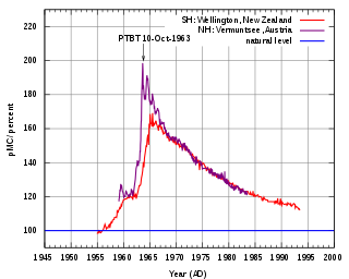
Effects of human activity

caption = Atmospheric
C for the northern and southern hemispheres, showing percentage excess above pre-bomb levels.  The Partial Test Ban Treaty went into effect on 10 October 1963.

Coal and oil began to be burned in large quantities during the 1800s. Both coal and oil are sufficiently old that they contain little detectable ¹⁴
C and, as a result, the CO
_² released substantially diluted the atmospheric ¹⁴
C/¹²
C ratio. Dating an object from the early 20th century hence gives an apparent date older than the true date. For the same reason, ¹⁴
C concentrations in the neighbourhood of large cities are lower than the atmospheric average. This fossil fuel effect (also known as the Suess effect, after Hans Suess, who first reported it in 1955) would only amount to a reduction of 0.2% in ¹⁴
C activity if the additional carbon from fossil fuels were distributed throughout the carbon exchange reservoir, but because of the long delay in mixing with the deep ocean, the actual effect is a 3% reduction. ^{[1] [11]}

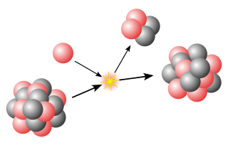
A much larger effect comes from above-ground nuclear testing, which released large numbers of neutrons and created ¹⁴
C. From about 1950 until 1963, when atmospheric nuclear testing was banned, it is estimated that several tonnes of ¹⁴
C were created. If all this extra ¹⁴
C had immediately been spread across the entire carbon exchange reservoir, it would have led to an increase in the ¹⁴
C/¹²
C ratio of only a few per cent, but the immediate effect was to almost double the amount of ¹⁴
C in the atmosphere, with the peak level occurring in about 1965. The level has since dropped, as the "bomb carbon" (as it is sometimes called) percolates into the rest of the reservoir. ^{[1] [11] [12]}

Isotopic fractionation

Photosynthesis is the primary process by which carbon moves from the atmosphere into living things. Two different photosynthetic processes exist: the C3 pathway and the C4 pathway. About 90% of all plant life uses the C3 process; the remaining plants either use C4 or are CAM plants, which can use either C3 or C4 depending on the environmental conditions. Both the C3 and C4 photosynthesis pathways show a preference for lighter carbon, with ¹²
C being absorbed slightly more easily than ¹³
C, which in turn is more easily absorbed than ¹⁴
C. The differential uptake of the three carbon isotopes leads to ¹³
C/¹²
C and ¹⁴
C/¹²
C ratios in plants that differ from the ratios in the atmosphere. This effect is known as isotopic fractionation. ^{[9] [13]}

To determine the degree of fractionation that takes place in a given plant, the amounts of both ¹²
C and ¹³
C are measured, and the resulting ¹³
C/¹²
C ratio is then compared to a standard ratio known as PDB. (The ¹³
C/¹²
C ratio is used because it is much easier to measure than the ¹⁴
C/¹²
C ratio, and the ¹⁴
C/¹²
C ratio can be easily derived from it.) The resulting value, known as δ¹³C, is calculated as follows: ^[9]

${\displaystyle {\ce {\delta ^{13}C}}=\left({\frac {\left({\frac {{\ce {^{13}C}}}{{\ce {^{12}C}}}}\right)_{{\ce {sample}}}}{\left({\frac {{\ce {^{13}C}}}{{\ce {^{12}C}}}}\right)_{{\ce {PDB}}}}}-1\right)\times 1000}$ ‰

where the ‰ (permil) sign indicates parts per thousand. ^[9] Because the PDB standard contains an unusually high proportion of ¹³
C, ^{[note 2]} most measured δ¹³C _{values are negative. Values for C3 plants typically range from −30‰ to −22‰, with an average of −27‰; for C4 plants the range is −15‰ to −9‰, and the average is −13‰. ^[13] Atmospheric CO
² has a δ¹³C of −8‰. ^[9]}

Sheep on the beach in North Ronaldsay. In the winter, these sheep eat seaweed, which has a higher δC _{content than grass; samples from these sheep have a δC value of about −13‰, which is much higher than for sheep that feed on grasses.}

For marine organisms, the details of the photosynthesis reactions are less well understood. Measured δ¹³C _{values for marine plankton range from −31‰ to −10‰; most lie between −22‰ and −17‰. The δ¹³C values for marine photosynthetic organisms also depend on temperature. At higher temperatures, CO
² has poor solubility in water, which means there is less CO
² available for the photosynthetic reactions. Under these conditions, fractionation is reduced, and at temperatures above 14 °C the δ¹³C values are correspondingly higher, reaching −13‰. At lower temperatures, CO
² becomes more soluble and hence more available to the marine organisms; fractionation increases and δ¹³C values can be as low as −32‰. ^[13]}

The δ¹³C _{value for animals depends on their diet. An animal that eats food with high δ¹³C values will have a higher δ¹³C than one that eats food with lower δ¹³C values. ^[9] The animal's own biochemical processes can also affect the results: for example, both bone minerals and bone collagen typically have a higher concentration of ¹³
C than is found in the animal's diet, though for different biochemical reasons. The enrichment of bone ¹³
C also implies that excreted material is depleted in ¹³
C relative to the diet. ^[15]}

Since ¹³
C makes up about 1% of the carbon in a sample, the ¹³
C/¹²
C ratio can be accurately measured by mass spectrometry. ^[16] Typical values of δ¹³C _{have been found by experiment for many plants, as well as for different parts of animals such as bone collagen, but when dating a given sample it is better to determine the δ¹³C value for that sample directly than to rely on the published values. ^[9] The depletion of ¹³
C relative to ¹²
C is proportional to the difference in the atomic masses of the two isotopes, so once the δ¹³C value is known, the depletion for ¹⁴
C can be calculated: it will be twice the depletion of ¹³
C. ^[16]}

The carbon exchange between atmospheric CO
_² and carbonate at the ocean surface is also subject to fractionation, with ¹⁴
C in the atmosphere more likely than ¹²
C to dissolve in the ocean. The result is an overall increase in the ¹⁴
C/¹²
C ratio in the ocean of 1.5%, relative to the ¹⁴
C/¹²
C ratio in the atmosphere. This increase in ¹⁴
C concentration almost exactly cancels out the decrease caused by the upwelling of water (containing old, and hence ¹⁴
C depleted, carbon) from the deep ocean, so that direct measurements of ¹⁴
C radiation are similar to measurements for the rest of the biosphere. Correcting for isotopic fractionation, as is done for all radiocarbon dates to allow comparison between results from different parts of the biosphere, gives an apparent age of about 400 years for ocean surface water. ^[16]

Reservoir effects

Libby's original exchange reservoir hypothesis assumed that the ¹⁴
C/¹²
C ratio in the exchange reservoir is constant all over the world, ^[17] but it has since been discovered that there are several causes of variation in the ratio across the reservoir. ^[18]

Marine effect

The CO
_² in the atmosphere transfers to the ocean by dissolving in the surface water as carbonate and bicarbonate ions; at the same time the carbonate ions in the water are returning to the air as CO
_². ^[17] This exchange process brings¹⁴
C from the atmosphere into the surface waters of the ocean, but the ¹⁴
C thus introduced takes a long time to percolate through the entire volume of the ocean. The deepest parts of the ocean mix very slowly with the surface waters, and the mixing is known to be uneven. The main mechanism that brings deep water to the surface is upwelling. Upwelling is more common in regions closer to the equator; it is also influenced by other factors such as the topography of the local ocean bottom and coastlines, the climate, and wind patterns. Overall, the mixing of deep and surface waters takes far longer than the mixing of atmospheric CO
_² with the surface waters, and as a result water from some deep ocean areas has an apparent radiocarbon age of several thousand years. Upwelling mixes this "old" water with the surface water, giving the surface water an apparent age of about several hundred years (after correcting for fractionation). ^[18] This effect is not uniform—the average effect is about 440 years, but there are local deviations of several hundred years for areas that are geographically close to each other. ^{[18] [19]} The effect also applies to marine organisms such as shells, and marine mammals such as whales and seals, which have radiocarbon ages that appear to be hundreds of years old. ^[18] These marine reservoir effects vary over time as well as geographically; for example, there is evidence that during the Younger Dryas, a period of cold climatic conditions about 12,000 years ago, the apparent difference between the age of surface water and the contemporary atmosphere increased from between 400 and 600 years to about 900 years until the climate warmed again. ^[19]

Hard water effect

If the carbon in freshwater is partly acquired from aged carbon, such as rocks, then the result will be a reduction in the ¹⁴
C/¹²
C ratio in the water. For example, rivers that pass over limestone, which is mostly composed of calcium carbonate, will acquire carbonate ions. Similarly, groundwater can contain carbon derived from the rocks through which it has passed. These rocks are usually so old that they no longer contain any measurable ¹⁴
C, so this carbon lowers the ¹⁴
C/¹²
C ratio of the water it enters, which can lead to apparent ages of thousands of years for both the affected water and the plants and freshwater organisms that live in it. ^[16] This is known as the hard water effect, because it is often associated with calcium ions, which are characteristic of hard water; however, there can be other sources of carbon that have the same effect, such as humus. The effect is not necessarily confined to freshwater species—at a river mouth, the outflow may affect marine organisms. It can also affect terrestrial snails that feed in areas where there is a high chalk content, though no measurable effect has been found for land plants in soil with a high carbonate content—it appears that almost all the carbon for these plants is derived from photosynthesis and not from the soil. ^[18]

It is not possible to deduce the effect of the effect by determining the hardness of the water: the aged carbon is not necessarily immediately incorporated into the plants and animals that are affected, and the delay affects their apparent age. The effect is very variable and there is no general offset that can be applied; the usual way to determine the size of the effect is to measure the apparent age offset of a modern sample. ^[18]

Volcanoes

Volcanic eruptions eject large amounts of carbon into the air. The carbon is of geological origin and has no detectable ¹⁴
C, so the ¹⁴
C/¹²
C ratio in the vicinity of the volcano is depressed relative to surrounding areas. Dormant volcanoes can also emit aged carbon. Plants that photosynthesize this carbon also have lower ¹⁴
C/¹²
C ratios: for example, plants on the Greek island of Santorini, near the volcano, have apparent ages of up to a thousand years. These effects are hard to predict—the town of Akrotiri, on Santorini, was destroyed in a volcanic eruption thousands of years ago, but radiocarbon dates for objects recovered from the ruins of the town show surprisingly close agreement with dates derived from other means. If the dates for Akrotiri are confirmed, it would indicate that the volcanic effect in this case was minimal. ^[18]

Hemisphere effect

The northern and southern hemispheres have atmospheric circulation systems that are sufficiently independent of each other that there is a noticeable time lag in mixing between the two. The atmospheric ¹⁴
C/¹²
C ratio is lower in the southern hemisphere, with an apparent additional age of 30 years for radiocarbon results from the south as compared to the north. This is probably because the greater surface area of ocean in the southern hemisphere means that there is more carbon exchanged between the ocean and the atmosphere than in the north. Since the surface ocean is depleted in ¹⁴
C because of the marine effect, ¹⁴
C is removed from the southern atmosphere more quickly than in the north. ^[18]

Island effect

It has been suggested that an "island effect" might exist, by analogy with the mechanism thought to explain the hemisphere effect: since islands are surrounded by water, the carbon exchange between the water and atmosphere might reduce the ¹⁴
C/¹²
C ratio on an island. Within a hemisphere, however, atmospheric mixing is apparently rapid enough that no such effect exists: two calibration curves assembled in Seattle and Belfast laboratories, with results from North American trees and Irish trees, respectively, are in close agreement, instead of the Irish samples appearing to be older, as would be the case if there were an island effect. ^[18]

Contamination

Any addition of carbon to a sample of a different age will cause the measured date to be inaccurate. Contamination with modern carbon causes a sample to appear to be younger than it really is: the effect is greater for older samples. If a sample that is in fact 17,000 years old is contaminated so that 1% of the sample is actually modern carbon, it will appear to be 600 years younger; for a sample that is 34,000 years old the same amount of contamination would cause an error of 4,000 years. Contamination with old carbon, with no remaining ¹⁴
C, causes an error in the other direction, which does not depend on age—a sample that has been contaminated with 1% old carbon will appear to be about 80 years older than it really is, regardless of the date of the sample. ^[20]

Contamination can occur if the sample is brought into contact with or packed in materials that contain carbon. Cotton wool, cigarette ash, paper labels, cloth bags, and some conservation chemicals such as polyvinyl acetate can all be sources of modern carbon. ^[21] Labels should be added to the outside of the container, not placed inside the bag or vial with the sample. Glass wool is acceptable as packing material instead of cotton wool. ^[22] Samples should be packed in glass vials or aluminium foil if possible; ^{[21] [23]} polyethylene bags are also acceptable but some plastics, such as PVC, can contaminate the sample. ^[22] Contamination can also occur before the sample is collected: humic acids or carbonate from the soil can leach into a sample, and for some sample types, such as shells, there is the possibility of carbon exchange between the sample and the environment, depleting the sample's ¹⁴
C content. ^[21]

Notes

1. Even at an altitude of 3 km, the neutron flux is only 3% of the value in the stratosphere where most ¹⁴
   C is created; at sea level the value is less than 0.5% of the value in the stratosphere. ^[9]
2. The PDB value is 11.1‰. ^[14]

Footnotes

1. Bowman (1995), pp. 16–20.
2. Suess (1970), p. 303.
3. Reimer, Paula J.; et al. (2013). "IntCal13 and Marine13 radiocarbon age calibration curves 0–50,000 years cal BP". Radiocarbon. 55 (4): 1869–1887. doi: 10.2458/azu_js_rc.55.16947 .
4. Bowman (1995), pp. 43–49.
5. Aitken (1990), pp. 68–69.
6. Rasskazov, Brandt & Brandt (2009), p. 40.
7. Grootes, Pieter M. (1992). "Subtle ¹⁴
   C Signals: The Influence of Atmospheric Mixing, Growing Season and In-Situ Production". Radiocarbon. 34 (2): 219–225. doi: 10.1017/S0033822200013655 .
8. Ramsey, C.B. (2008). "Radiocarbon dating: revolutions in understanding". Archaeometry. 50 (2): 249–275. doi:10.1111/j.1475-4754.2008.00394.x.
9. Bowman (1995), pp. 20–23.
10. Hua, Quan; Barbetti, Mike; Rakowski, Andrzej Z. (2013). "Atmospheric Radiocarbon for the Period 1950–2010". Radiocarbon. 55 (4): 2059–2072. doi: 10.2458/azu_js_rc.v55i2.16177 . ISSN   0033-8222.
11. Aitken (1990), pp. 71–72.
12. "Limited Test Ban Treaty". Science Magazine. Retrieved July 26, 2013.
13. Maslin & Swann (2006), p. 246.
14. Miller & Wheeler (2012), p. 186.
15. Schoeninger (2010), p. 446.
16. Aitken (1990), pp. 61–66.
17. Libby (1965), p. 6.
18. Bowman (1995), pp. 24–27.
19. Cronin (2010), p. 35.
20. Aitken (1990), pp. 85–86.
21. Bowman (1995), pp. 27–30.
22. Aitken (1990), p. 89.
23. Burke, Smith & Zimmerman (2009), p. 175.

References

• Aitken, M.J. (1990). Science-based Dating in Archaeology. London: Longman. ISBN   978-0-582-49309-4.
• Bowman, Sheridan (1995) [1990]. Radiocarbon Dating . London: British Museum Press. ISBN   978-0-7141-2047-8.
• Burke, Heather; Smith, Claire; Zimmerman, Larry J. (2009). The Archaeologist's Field Handbook (North American ed.). Lanham, MD: AltaMira Press. ISBN   978-0-7591-0882-0.
• Cronin, Thomas M. (2010). Paleoclimates: Understanding Climate Change Past and Present. New York: Columbia University Press. ISBN   978-0-231-14494-0.
• Šilar, Jan (2004). "Application of environmental radionuclides in radiochronology: Radiocarbon". In Tykva, Richard; Berg, Dieter (eds.). Man-made and Natural Radioactivity in Environmental Pollution and Radiochronology. Dordrecht: Kluwer Academic Publishers. pp. 150–179. ISBN   978-1-4020-1860-2.
• Libby, Willard F. (1965) [1952]. Radiocarbon Dating (2nd (1955) ed.). Chicago: Phoenix.
• Maslin, Mark A.; Swann, George E.A. (2006). "Isotopes in marine sediments". In Leng, Melanie J. (ed.). Isotopes in Palaeoenvironmental Research. Dordrecht: Springer. pp. 227–290. ISBN   978-1-4020-2503-7.
• Rasskazov, Sergei V.; Brandt, Sergei Borisovich; Brandt, Ivan S. (2009). Radiogenic Isotopes in Geologic Processes. Dordrecht: Springer. ISBN   978-90-481-2998-0.
• Schoeninger, Margaret J. (2010). "Diet reconstruction and ecology using stable isotope ratios". In Larsen, Clark Spencer (ed.). A Companion to Biological Anthropology. Oxford: Blackwell. pp. 445–464. ISBN   978-1-4051-8900-2.
• Suess, H.E. (1970). "Bristlecone-pine calibration of the radiocarbon time-scale 5200 B.C. to the present". In Olsson, Ingrid U. (ed.). Radiocarbon Variations and Absolute Chronology. New York: John Wiley & Sons. pp. 303–311.