Regularization by spectral filtering

Last updated May 02, 2024

Spectral regularization is any of a class of regularization techniques used in machine learning to control the impact of noise and prevent overfitting. Spectral regularization can be used in a broad range of applications, from deblurring images to classifying emails into a spam folder and a non-spam folder. For instance, in the email classification example, spectral regularization can be used to reduce the impact of noise and prevent overfitting when a machine learning system is being trained on a labeled set of emails to learn how to tell a spam and a non-spam email apart.

Spectral regularization algorithms rely on methods that were originally defined and studied in the theory of ill-posed inverse problems (for instance, see^[1]) focusing on the inversion of a linear operator (or a matrix) that possibly has a bad condition number or an unbounded inverse. In this context, regularization amounts to substituting the original operator by a bounded operator called the "regularization operator" that has a condition number controlled by a regularization parameter,^[2] a classical example being Tikhonov regularization. To ensure stability, this regularization parameter is tuned based on the level of noise.^[2] The main idea behind spectral regularization is that each regularization operator can be described using spectral calculus as an appropriate filter on the eigenvalues of the operator that defines the problem, and the role of the filter is to "suppress the oscillatory behavior corresponding to small eigenvalues".^[2] Therefore, each algorithm in the class of spectral regularization algorithms is defined by a suitable filter function (which needs to be derived for that particular algorithm). Three of the most commonly used regularization algorithms for which spectral filtering is well-studied are Tikhonov regularization, Landweber iteration, and truncated singular value decomposition (TSVD). As for choosing the regularization parameter, examples of candidate methods to compute this parameter include the discrepancy principle, generalized cross validation, and the L-curve criterion.^[3]

It is of note that the notion of spectral filtering studied in the context of machine learning is closely connected to the literature on function approximation (in signal processing).

Notation

The training set is defined as $S=\{(x_{1},y_{1}),\dots ,(x_{n},y_{n})\}$ , where $X$ is the $n\times d$ input matrix and $Y=(y_{1},\dots ,y_{n})$ is the output vector. Where applicable, the kernel function is denoted by $k$ , and the $n\times n$ kernel matrix is denoted by $K$ which has entries $K_{ij}=k(x_{i},x_{j})$ and ${\mathcal {H}}$ denotes the Reproducing Kernel Hilbert Space (RKHS) with kernel $k$ . The regularization parameter is denoted by $\lambda$ .

(Note: For $g\in G$ and $f\in F$ , with $G$ and $F$ being Hilbert spaces, given a linear, continuous operator $L$ , assume that $g=Lf$ holds. In this setting, the direct problem would be to solve for $g$ given $f$ and the inverse problem would be to solve for $f$ given $g$ . If the solution exists, is unique and stable, the inverse problem (i.e. the problem of solving for $f$ ) is well-posed; otherwise, it is ill-posed.)

Relation to the theory of ill-posed inverse problems

The connection between the regularized least squares (RLS) estimation problem (Tikhonov regularization setting) and the theory of ill-posed inverse problems is an example of how spectral regularization algorithms are related to the theory of ill-posed inverse problems.

The RLS estimator solves

\min _{f\in {\mathcal {H}}}{\frac {1}{n}}\sum _{i=1}^{n}(y_{i}-f(x_{i}))^{2}+\lambda \left\|f\right\|_{\mathcal {H}}^{2}

and the RKHS allows for expressing this RLS estimator as $f_{S}^{\lambda }(X)=\sum _{i=1}^{n}c_{i}k(x,x_{i})$ where $(K+n\lambda I)c=Y$ with $c=(c_{1},\dots ,c_{n})$ .^[4] The penalization term is used for controlling smoothness and preventing overfitting. Since the solution of empirical risk minimization $\min _{f\in {\mathcal {H}}}{\frac {1}{n}}\sum _{i=1}^{n}(y_{i}-f(x_{i}))^{2}$ can be written as $f_{S}^{\lambda }(X)=\sum _{i=1}^{n}c_{i}k(x,x_{i})$ such that $Kc=Y$ , adding the penalty function amounts to the following change in the system that needs to be solved:^[5]

\left\{\min _{f\in {\mathcal {H}}}{\frac {1}{n}}\sum _{i=1}^{n}\left(y_{i}-f(x_{i})\right)^{2}\rightarrow \min _{f\in {\mathcal {H}}}{\frac {1}{n}}\sum _{i=1}^{n}\left(y_{i}-f(x_{i})\right)^{2}+\lambda \left\|f\right\|_{\mathcal {H}}^{2}\right\}\equiv {\biggl \{}Kc=Y\rightarrow \left(K+n\lambda I\right)c=Y{\biggr \}}.

In this learning setting, the kernel matrix can be decomposed as $K=Q\Sigma Q^{T}$ , with

\sigma =\operatorname {diag} (\sigma _{1},\dots ,\sigma _{n}),~\sigma _{1}\geq \sigma _{2}\geq \cdots \geq \sigma _{n}\geq 0

and $q_{1},\dots ,q_{n}$ are the corresponding eigenvectors. Therefore, in the initial learning setting, the following holds:

c=K^{-1}Y=Q\Sigma ^{-1}Q^{T}Y=\sum _{i=1}^{n}{\frac {1}{\sigma _{i}}}\langle q_{i},Y\rangle q_{i}.

Thus, for small eigenvalues, even small perturbations in the data can lead to considerable changes in the solution. Hence, the problem is ill-conditioned, and solving this RLS problem amounts to stabilizing a possibly ill-conditioned matrix inversion problem, which is studied in the theory of ill-posed inverse problems; in both problems, a main concern is to deal with the issue of numerical stability.

Implementation of algorithms

Each algorithm in the class of spectral regularization algorithms is defined by a suitable filter function, denoted here by $G_{\lambda }(\cdot )$ . If the Kernel matrix is denoted by $K$ , then $\lambda$ should control the magnitude of the smaller eigenvalues of $G_{\lambda }(K)$ . In a filtering setup, the goal is to find estimators $f_{S}^{\lambda }(X):=\sum _{i=1}^{n}c_{i}k(x,x_{i})$ where $c=G_{\lambda }(K)Y$ . To do so, a scalar filter function $G_{\lambda }(\sigma )$ is defined using the eigen-decomposition of the kernel matrix:

G_{\lambda }(K)=QG_{\lambda }(\Sigma )Q^{T},

which yields

G_{\lambda }(K)Y~=~\sum _{i=1}^{n}G_{\lambda }(\sigma _{i})\langle q_{i},Y\rangle q_{i}.

Typically, an appropriate filter function should have the following properties:^[5]

As $\lambda$ goes to zero, $G_{\lambda }(\sigma )~\rightarrow ~1/\sigma$ .
The magnitude of the (smaller) eigenvalues of $G_{\lambda }$ is controlled by $\lambda$ .

While the above items give a rough characterization of the general properties of filter functions for all spectral regularization algorithms, the derivation of the filter function (and hence its exact form) varies depending on the specific regularization method that spectral filtering is applied to.

Filter function for Tikhonov regularization

In the Tikhonov regularization setting, the filter function for RLS is described below. As shown in,^[4] in this setting, $c=\left(K+n\lambda I\right)^{-1}Y$ . Thus,

c=(K+n\lambda I)^{-1}Y=Q(\Sigma +n\lambda I)^{-1}Q^{T}Y=\sum _{i=1}^{n}{\frac {1}{\sigma _{i}+n\lambda }}<q_{i},Y>q_{i}.

The undesired components are filtered out using regularization:

If $\sigma \gg \lambda n$ , then ${\frac {1}{\sigma _{i}+n\lambda }}\sim {\frac {1}{\sigma _{i}}}$ .
If $\sigma \ll \lambda n$ , then ${\frac {1}{\sigma _{i}+n\lambda }}\sim {\frac {1}{\lambda n}}$ .

The filter function for Tikhonov regularization is therefore defined as:^[5]

G_{\lambda }(\sigma )={\frac {1}{\sigma +n\lambda }}.

Filter function for Landweber iteration

The idea behind the Landweber iteration is gradient descent:^[5]

c⁰ := 0 fori = 1, ..., t − 1     cⁱ := cⁱ⁻¹ + η(Y − Kcⁱ⁻¹) end

In this setting, if $n$ is larger than $K$ 's largest eigenvalue, the above iteration converges by choosing $\eta =2/n$ as the step-size:.^[5] The above iteration is equivalent to minimizing ${\frac {1}{n}}\left\|Y-Kc\right\|_{2}^{2}$ (i.e. the empirical risk) via gradient descent; using induction, it can be proved that at the $t$ -th iteration, the solution is given by ^[5]

c=\eta \sum _{i=0}^{t-1}\left(I-\eta K\right)^{i}Y.

Thus, the appropriate filter function is defined by:

G_{\lambda }(\sigma )=\eta \sum _{i=0}^{t-1}\left(I-\eta \sigma \right)^{i}.

It can be shown that this filter function corresponds to a truncated power expansion of $K^{-1}$ ;^[5] to see this, note that the relation $\sum _{i\geq 0}x^{i}=1/(1-x)$ , would still hold if $x$ is replaced by a matrix; thus, if $K$ (the kernel matrix), or rather $I-\eta K$ , is considered, the following holds:

K^{-1}=\eta \sum _{i=0}^{\infty }\left(I-\eta K\right)^{i}\sim \eta \sum _{i=0}^{t-1}\left(I-\eta K\right)^{i}.

In this setting, the number of iterations gives the regularization parameter; roughly speaking, $t\sim 1/\lambda$ .^[5] If $t$ is large, overfitting may be a concern. If $t$ is small, oversmoothing may be a concern. Thus, choosing an appropriate time for early stopping of the iterations provides a regularization effect.

Filter function for TSVD

In the TSVD setting, given the eigen-decomposition $K=Q\Sigma Q^{T}$ and using a prescribed threshold $\lambda n$ , a regularized inverse can be formed for the kernel matrix by discarding all the eigenvalues that are smaller than this threshold.^[5] Thus, the filter function for TSVD can be defined as

G_{\lambda }(\sigma )={\begin{cases}1/\sigma ,&{\text{if }}\sigma \geq \lambda n\\[1ex]0,&{\text{otherwise}}\end{cases}}

It can be shown that TSVD is equivalent to the (unsupervised) projection of the data using (kernel) Principal Component Analysis (PCA), and that it is also equivalent to minimizing the empirical risk on the projected data (without regularization).^[5] Note that the number of components kept for the projection is the only free parameter here.

Related Research Articles

In physics and mathematics, the Lorentz group is the group of all Lorentz transformations of Minkowski spacetime, the classical and quantum setting for all (non-gravitational) physical phenomena. The Lorentz group is named for the Dutch physicist Hendrik Lorentz.

In mathematics, a Gaussian function, often simply referred to as a Gaussian, is a function of the base form

In statistics, Cochran's theorem, devised by William G. Cochran, is a theorem used to justify results relating to the probability distributions of statistics that are used in the analysis of variance.

Ridge regression is a method of estimating the coefficients of multiple-regression models in scenarios where the independent variables are highly correlated. It has been used in many fields including econometrics, chemistry, and engineering. Also known as Tikhonov regularization, named for Andrey Tikhonov, it is a method of regularization of ill-posed problems. It is particularly useful to mitigate the problem of multicollinearity in linear regression, which commonly occurs in models with large numbers of parameters. In general, the method provides improved efficiency in parameter estimation problems in exchange for a tolerable amount of bias.

In mathematics, the Weierstrass functions are special functions of a complex variable that are auxiliary to the Weierstrass elliptic function. They are named for Karl Weierstrass. The relation between the sigma, zeta, and $functions is analogous to that between the sine, cotangent, and squared cosecant functions: the logarithmic derivative of the sine is the cotangent, whose derivative is negative the squared cosecant.$

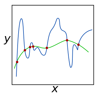
<span class="mw-page-title-main">Regularization (mathematics)</span> Technique to make a model more generalizable and transferable

In mathematics, statistics, finance, and computer science, particularly in machine learning and inverse problems, regularization is a process that changes the result answer to be "simpler". It is often used to obtain results for ill-posed problems or to prevent overfitting.

The quantum Heisenberg model, developed by Werner Heisenberg, is a statistical mechanical model used in the study of critical points and phase transitions of magnetic systems, in which the spins of the magnetic systems are treated quantum mechanically. It is related to the prototypical Ising model, where at each site of a lattice, a spin $represents a microscopic magnetic dipole to which the magnetic moment is either up or down. Except the coupling between magnetic dipole moments, there is also a multipolar version of Heisenberg model called the multipolar exchange interaction.$

In the mathematical discipline of functional analysis, the concept of a compact operator on Hilbert space is an extension of the concept of a matrix acting on a finite-dimensional vector space; in Hilbert space, compact operators are precisely the closure of finite-rank operators in the topology induced by the operator norm. As such, results from matrix theory can sometimes be extended to compact operators using similar arguments. By contrast, the study of general operators on infinite-dimensional spaces often requires a genuinely different approach.

Covariance matrix adaptation evolution strategy (CMA-ES) is a particular kind of strategy for numerical optimization. Evolution strategies (ES) are stochastic, derivative-free methods for numerical optimization of non-linear or non-convex continuous optimization problems. They belong to the class of evolutionary algorithms and evolutionary computation. An evolutionary algorithm is broadly based on the principle of biological evolution, namely the repeated interplay of variation and selection: in each generation (iteration) new individuals are generated by variation, usually in a stochastic way, of the current parental individuals. Then, some individuals are selected to become the parents in the next generation based on their fitness or objective function value $. Like this, over the generation sequence, individuals with better and better -values are generated.$

In mathematics and mathematical physics, raising and lowering indices are operations on tensors which change their type. Raising and lowering indices are a form of index manipulation in tensor expressions.

In mathematics, every analytic function can be used for defining a matrix function that maps square matrices with complex entries to square matrices of the same size.

In the fields of computer vision and image analysis, the Harris affine region detector belongs to the category of feature detection. Feature detection is a preprocessing step of several algorithms that rely on identifying characteristic points or interest points so to make correspondences between images, recognize textures, categorize objects or build panoramas.

In mathematics, the spectral theory of ordinary differential equations is the part of spectral theory concerned with the determination of the spectrum and eigenfunction expansion associated with a linear ordinary differential equation. In his dissertation, Hermann Weyl generalized the classical Sturm–Liouville theory on a finite closed interval to second order differential operators with singularities at the endpoints of the interval, possibly semi-infinite or infinite. Unlike the classical case, the spectrum may no longer consist of just a countable set of eigenvalues, but may also contain a continuous part. In this case the eigenfunction expansion involves an integral over the continuous part with respect to a spectral measure, given by the Titchmarsh–Kodaira formula. The theory was put in its final simplified form for singular differential equations of even degree by Kodaira and others, using von Neumann's spectral theorem. It has had important applications in quantum mechanics, operator theory and harmonic analysis on semisimple Lie groups.

In computer science, online machine learning is a method of machine learning in which data becomes available in a sequential order and is used to update the best predictor for future data at each step, as opposed to batch learning techniques which generate the best predictor by learning on the entire training data set at once. Online learning is a common technique used in areas of machine learning where it is computationally infeasible to train over the entire dataset, requiring the need of out-of-core algorithms. It is also used in situations where it is necessary for the algorithm to dynamically adapt to new patterns in the data, or when the data itself is generated as a function of time, e.g., stock price prediction. Online learning algorithms may be prone to catastrophic interference, a problem that can be addressed by incremental learning approaches.

Within bayesian statistics for machine learning, kernel methods arise from the assumption of an inner product space or similarity structure on inputs. For some such methods, such as support vector machines (SVMs), the original formulation and its regularization were not Bayesian in nature. It is helpful to understand them from a Bayesian perspective. Because the kernels are not necessarily positive semidefinite, the underlying structure may not be inner product spaces, but instead more general reproducing kernel Hilbert spaces. In Bayesian probability kernel methods are a key component of Gaussian processes, where the kernel function is known as the covariance function. Kernel methods have traditionally been used in supervised learning problems where the input space is usually a space of vectors while the output space is a space of scalars. More recently these methods have been extended to problems that deal with multiple outputs such as in multi-task learning.

In machine learning, the kernel embedding of distributions comprises a class of nonparametric methods in which a probability distribution is represented as an element of a reproducing kernel Hilbert space (RKHS). A generalization of the individual data-point feature mapping done in classical kernel methods, the embedding of distributions into infinite-dimensional feature spaces can preserve all of the statistical features of arbitrary distributions, while allowing one to compare and manipulate distributions using Hilbert space operations such as inner products, distances, projections, linear transformations, and spectral analysis. This learning framework is very general and can be applied to distributions over any space $on which a sensible kernel function may be defined. For example, various kernels have been proposed for learning from data which are: vectors in, discrete classes/categories, strings, graphs/networks, images, time series, manifolds, dynamical systems, and other structured objects. The theory behind kernel embeddings of distributions has been primarily developed by Alex Smola, Le Song, Arthur Gretton, and Bernhard Schölkopf. A review of recent works on kernel embedding of distributions can be found in.$

In the field of statistical learning theory, matrix regularization generalizes notions of vector regularization to cases where the object to be learned is a matrix. The purpose of regularization is to enforce conditions, for example sparsity or smoothness, that can produce stable predictive functions. For example, in the more common vector framework, Tikhonov regularization optimizes over

Regularized least squares (RLS) is a family of methods for solving the least-squares problem while using regularization to further constrain the resulting solution.

Low-rank matrix approximations are essential tools in the application of kernel methods to large-scale learning problems.

The quaternion estimator algorithm (QUEST) is an algorithm designed to solve Wahba's problem, that consists of finding a rotation matrix between two coordinate systems from two sets of observations sampled in each system respectively. The key idea behind the algorithm is to find an expression of the loss function for the Wahba's problem as a quadratic form, using the Cayley–Hamilton theorem and the Newton–Raphson method to efficiently solve the eigenvalue problem and construct a numerically stable representation of the solution.

References

↑ H. W. Engl, M. Hanke, and A. Neubauer. Regularization of inverse problems. Kluwer, 1996.
1 2 3 L. Lo Gerfo, L. Rosasco, F. Odone, E. De Vito, and A. Verri. Spectral Algorithms for Supervised Learning, Neural Computation, 20(7), 2008.
↑ P. C. Hansen, J. G. Nagy, and D. P. O'Leary. Deblurring Images: Matrices, Spectra, and Filtering, Fundamentals of Algorithms 3, SIAM, Philadelphia, 2006.
1 2 L. Rosasco. Lecture 6 of the Lecture Notes for 9.520: Statistical Learning Theory and Applications. Massachusetts Institute of Technology, Fall 2013. Available at https://www.mit.edu/~9.520/fall13/slides/class06/class06_RLSSVM.pdf
1 2 3 4 5 6 7 8 9 10 L. Rosasco. Lecture 7 of the Lecture Notes for 9.520: Statistical Learning Theory and Applications. Massachusetts Institute of Technology, Fall 2013. Available at https://www.mit.edu/~9.520/fall13/slides/class07/class07_spectral.pdf

This page is based on this Wikipedia article
Text is available under the CC BY-SA 4.0 license; additional terms may apply.
Images, videos and audio are available under their respective licenses.

[1] H. W. Engl, M. Hanke, and A. Neubauer. Regularization of inverse problems. Kluwer, 1996.

[rosasco-2] 1 2 3 L. Lo Gerfo, L. Rosasco, F. Odone, E. De Vito, and A. Verri. Spectral Algorithms for Supervised Learning, Neural Computation, 20(7), 2008.

[3] P. C. Hansen, J. G. Nagy, and D. P. O'Leary. Deblurring Images: Matrices, Spectra, and Filtering, Fundamentals of Algorithms 3, SIAM, Philadelphia, 2006.

[BB-4] 1 2 L. Rosasco. Lecture 6 of the Lecture Notes for 9.520: Statistical Learning Theory and Applications. Massachusetts Institute of Technology, Fall 2013. Available at https://www.mit.edu/~9.520/fall13/slides/class06/class06_RLSSVM.pdf

[AA-5] 1 2 3 4 5 6 7 8 9 10 L. Rosasco. Lecture 7 of the Lecture Notes for 9.520: Statistical Learning Theory and Applications. Massachusetts Institute of Technology, Fall 2013. Available at https://www.mit.edu/~9.520/fall13/slides/class07/class07_spectral.pdf

[1]

[2]

[3]

[4]

[5]