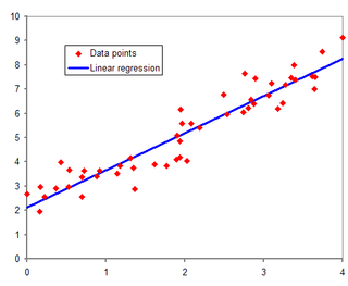
The method of least squares is a standard approach in regression analysis to approximate the solution of overdetermined systems by minimizing the sum of the squares of the residuals made in the results of each individual equation.
In statistics, the Gauss–Markov theorem states that the ordinary least squares (OLS) estimator has the lowest sampling variance within the class of linear unbiased estimators, if the errors in the linear regression model are uncorrelated, have equal variances and expectation value of zero. The errors do not need to be normal, nor do they need to be independent and identically distributed. The requirement that the estimator be unbiased cannot be dropped, since biased estimators exist with lower variance. See, for example, the James–Stein estimator, ridge regression, or simply any degenerate estimator.

In statistics, Deming regression, named after W. Edwards Deming, is an errors-in-variables model which tries to find the line of best fit for a two-dimensional dataset. It differs from the simple linear regression in that it accounts for errors in observations on both the x- and the y- axis. It is a special case of total least squares, which allows for any number of predictors and a more complicated error structure.
In statistics, a studentized residual is the quotient resulting from the division of a residual by an estimate of its standard deviation. It is a form of a Student's t-statistic, with the estimate of error varying between points.

In statistical modeling, regression analysis is a set of statistical processes for estimating the relationships between a dependent variable and one or more independent variables. The most common form of regression analysis is linear regression, in which one finds the line that most closely fits the data according to a specific mathematical criterion. For example, the method of ordinary least squares computes the unique line that minimizes the sum of squared differences between the true data and that line. For specific mathematical reasons, this allows the researcher to estimate the conditional expectation of the dependent variable when the independent variables take on a given set of values. Less common forms of regression use slightly different procedures to estimate alternative location parameters or estimate the conditional expectation across a broader collection of non-linear models.

In applied statistics, total least squares is a type of errors-in-variables regression, a least squares data modeling technique in which observational errors on both dependent and independent variables are taken into account. It is a generalization of Deming regression and also of orthogonal regression, and can be applied to both linear and non-linear models.

In statistics, the coefficient of determination, denoted R2 or r2 and pronounced "R squared", is the proportion of the variation in the dependent variable that is predictable from the independent variable(s).
In statistics, ordinary least squares (OLS) is a type of linear least squares method for choosing the unknown parameters in a linear regression model by the principle of least squares: minimizing the sum of the squares of the differences between the observed dependent variable in the input dataset and the output of the (linear) function of the independent variable.
In statistics, the number of degrees of freedom is the number of values in the final calculation of a statistic that are free to vary.
In statistics, the explained sum of squares (ESS), alternatively known as the model sum of squares or sum of squares due to regression, is a quantity used in describing how well a model, often a regression model, represents the data being modelled. In particular, the explained sum of squares measures how much variation there is in the modelled values and this is compared to the total sum of squares (TSS), which measures how much variation there is in the observed data, and to the residual sum of squares, which measures the variation in the error between the observed data and modelled values.

In statistics, simple linear regression is a linear regression model with a single explanatory variable. That is, it concerns two-dimensional sample points with one independent variable and one dependent variable and finds a linear function that, as accurately as possible, predicts the dependent variable values as a function of the independent variable. The adjective simple refers to the fact that the outcome variable is related to a single predictor.
In statistics, generalized least squares (GLS) is a technique for estimating the unknown parameters in a linear regression model when there is a certain degree of correlation between the residuals in a regression model. In these cases, ordinary least squares and weighted least squares can be statistically inefficient, or even give misleading inferences. GLS was first described by Alexander Aitken in 1936.
In statistics, the Durbin–Watson statistic is a test statistic used to detect the presence of autocorrelation at lag 1 in the residuals from a regression analysis. It is named after James Durbin and Geoffrey Watson. The small sample distribution of this ratio was derived by John von Neumann. Durbin and Watson applied this statistic to the residuals from least squares regressions, and developed bounds tests for the null hypothesis that the errors are serially uncorrelated against the alternative that they follow a first order autoregressive process. Note that the distribution of this test statistic does not depend on the estimated regression coefficients and the variance of the errors.
In probability theory and statistics, partial correlation measures the degree of association between two random variables, with the effect of a set of controlling random variables removed. When determining the numerical relationship between two variables of interest, using their correlation coefficient will give misleading results if there is another confounding variable that is numerically related to both variables of interest. This misleading information can be avoided by controlling for the confounding variable, which is done by computing the partial correlation coefficient. This is precisely the motivation for including other right-side variables in a multiple regression; but while multiple regression gives unbiased results for the effect size, it does not give a numerical value of a measure of the strength of the relationship between the two variables of interest.
The topic of heteroskedasticity-consistent (HC) standard errors arises in statistics and econometrics in the context of linear regression and time series analysis. These are also known as heteroskedasticity-robust standard errors, Eicker–Huber–White standard errors, to recognize the contributions of Friedhelm Eicker, Peter J. Huber, and Halbert White.
In statistics, the variance inflation factor (VIF) is the ratio (quotient) of the variance of estimating some parameter in a model that includes multiple other terms (parameters) by the variance of a model constructed using only one term. It quantifies the severity of multicollinearity in an ordinary least squares regression analysis. It provides an index that measures how much the variance of an estimated regression coefficient is increased because of collinearity. Cuthbert Daniel claims to have invented the concept behind the variance inflation factor, but did not come up with the name.
In linear regression, mean response and predicted response are values of the dependent variable calculated from the regression parameters and a given value of the independent variable. The values of these two responses are the same, but their calculated variances are different.
In statistics, principal component regression (PCR) is a regression analysis technique that is based on principal component analysis (PCA). More specifically, PCR is used for estimating the unknown regression coefficients in a standard linear regression model.
In statistics and in particular in regression analysis, leverage is a measure of how far away the independent variable values of an observation are from those of the other observations. High-leverage points, if any, are outliers with respect to the independent variables. That is, high-leverage points have no neighboring points in space, where is the number of independent variables in a regression model. This makes the fitted model likely to pass close to a high leverage observation. Hence high-leverage points have the potential to cause large changes in the parameter estimates when they are deleted i.e., to be influential points. Although an influential point will typically have high leverage, a high leverage point is not necessarily an influential point. The leverage is typically defined as the diagonal elements of the hat matrix.
The purpose of this page is to provide supplementary materials for the ordinary least squares article, reducing the load of the main article with mathematics and improving its accessibility, while at the same time retaining the completeness of exposition.


