Sensitivity (control systems)

Last updated June 01, 2023

In control engineering, the sensitivity (or more precisely, the sensitivity function) of a control system measures how variations in the plant parameters affects the closed-loop transfer function. Since the controller parameters are typically matched to the process characteristics and the process may change, it is important that the controller parameters are chosen in such a way that the closed loop system is not sensitive to variations in process dynamics. Moreover, the sensitivity function is also important to analyse how disturbances affects the system.

Sensitivity function

A basic closed loop control system, using unity negative feedback. C(s) and G(s) denote compensator and plant transfer functions, respectively.

Let $G(s)$ and $C(s)$ denote the plant and controller's transfer function in a basic closed loop control system written in the Laplace domain using unity negative feedback.

Sensitivity function as a measure of robustness to parameter variation

The closed-loop transfer function is given by

$T(s)={\frac {G(s)C(s)}{1+G(s)C(s)}}.$

Differentiating $T$ with respect to $G$ yields

${\frac {dT}{dG}}={\frac {d}{dG}}\left[{\frac {GC}{1+GC}}\right]={\frac {C}{(1+CG)^{2}}}=S{\frac {T}{G}},$

where $S$ is defined as the function

$S(s)={\frac {1}{1+G(s)C(s)}}$

and is known as the sensitivity function. Lower values of $|S|$ implies that relative errors in the plant parameters has less effects in the relative error of the closed-loop transfer function.

Sensitivity function as a measure of disturbance attenuation

The sensitivity function also describes the transfer function from external disturbance to process output. In fact, assuming an additive disturbance n after the output

of the plant, the transfer functions of the closed loop system are given by

$Y(s)={\frac {C(s)G(s)}{1+C(s)G(s)}}R(s)+{\frac {1}{1+C(s)G(s)}}N(s).$

Hence, lower values of $|S|$ suggest further attenuation of the external disturbance. The sensitivity function tells us how the disturbances are influenced by feedback. Disturbances with frequencies such that $|S(j\omega )|$ is less than one are reduced by an amount equal to the distance to the critical point $-1$ and disturbances with frequencies such that $|S(j\omega )|$ is larger than one are amplified by the feedback.^[1]

Sensitivity peak and sensitivity circle

Sensitivity peak

It is important that the largest value of the sensitivity function be limited for a control system. The nominal sensitivity peak $M_{s}$ is defined as^[2]

$M_{s}=\max _{0\leq \omega <\infty }\left|S(j\omega )\right|=\max _{0\leq \omega <\infty }\left|{\frac {1}{1+G(j\omega )C(j\omega )}}\right|$

and it is common to require that the maximum value of the sensitivity function, $M_{s}$ , be in a range of 1.3 to 2.

Sensitivity circle

The quantity $M_{s}$ is the inverse of the shortest distance from the Nyquist curve of the loop transfer function to the critical point $-1$ . A sensitivity $M_{s}$ guarantees that the distance from the critical point to the Nyquist curve is always greater than ${\frac {1}{M_{s}}}$ and the Nyquist curve of the loop transfer function is always outside a circle around the critical point $-1+0j$ with the radius ${\frac {1}{M_{s}}}$ , known as the sensitivity circle. $M_{s}$ defines the maximum value of the sensitivity function and the inverse of $M_{s}$ gives you the shortest distance from the open-loop transfer function $L(j\omega )$ to the critical point $-1+0j$ .^[3]^[4]

Related Research Articles

Control theory is a field of control engineering and applied mathematics that deals with the control of dynamical systems in engineered processes and machines. The objective is to develop a model or algorithm governing the application of system inputs to drive the system to a desired state, while minimizing any delay, overshoot, or steady-state error and ensuring a level of control stability; often with the aim to achieve a degree of optimality.

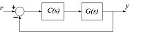
In engineering, a transfer function of a system, sub-system, or component is a mathematical function that models the system's output for each possible input. They are widely used in electronic engineering tools like circuit simulators and control systems. In some simple cases, this function is a two-dimensional graph of an independent scalar input versus the dependent scalar output, called a transfer curve or characteristic curve. Transfer functions for components are used to design and analyze systems assembled from components, particularly using the block diagram technique, in electronics and control theory.

A phase-locked loop or phase lock loop (PLL) is a control system that generates an output signal whose phase is related to the phase of an input signal. There are several different types; the simplest is an electronic circuit consisting of a variable frequency oscillator and a phase detector in a feedback loop. The oscillator's frequency and phase are controlled proportionally by an applied voltage, hence the term voltage-controlled oscillator (VCO). The oscillator generates a periodic signal of a specific frequency, and the phase detector compares the phase of that signal with the phase of the input periodic signal, to adjust the oscillator to keep the phases matched.

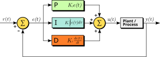
A proportional–integral–derivative controller is a control loop mechanism employing feedback that is widely used in industrial control systems and a variety of other applications requiring continuously modulated control. A PID controller continuously calculates an error value $as the difference between a desired setpoint (SP) and a measured process variable (PV) and applies a correction based on proportional, integral, and derivative terms, hence the name.$

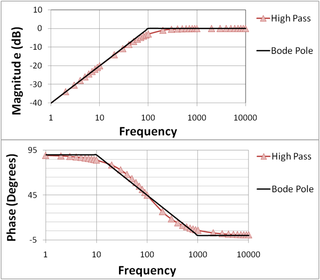
In electrical engineering and control theory, a Bode plot is a graph of the frequency response of a system. It is usually a combination of a Bode magnitude plot, expressing the magnitude of the frequency response, and a Bode phase plot, expressing the phase shift.

Negative feedback occurs when some function of the output of a system, process, or mechanism is fed back in a manner that tends to reduce the fluctuations in the output, whether caused by changes in the input or by other disturbances.

H_∞methods are used in control theory to synthesize controllers to achieve stabilization with guaranteed performance. To use H_∞ methods, a control designer expresses the control problem as a mathematical optimization problem and then finds the controller that solves this optimization. H_∞ techniques have the advantage over classical control techniques in that H_∞ techniques are readily applicable to problems involving multivariate systems with cross-coupling between channels; disadvantages of H_∞ techniques include the level of mathematical understanding needed to apply them successfully and the need for a reasonably good model of the system to be controlled. It is important to keep in mind that the resulting controller is only optimal with respect to the prescribed cost function and does not necessarily represent the best controller in terms of the usual performance measures used to evaluate controllers such as settling time, energy expended, etc. Also, non-linear constraints such as saturation are generally not well-handled. These methods were introduced into control theory in the late 1970s-early 1980s by George Zames, J. William Helton , and Allen Tannenbaum.

<span class="mw-page-title-main">Root locus analysis</span> Stability criterion in control theory

In control theory and stability theory, root locus analysis is a graphical method for examining how the roots of a system change with variation of a certain system parameter, commonly a gain within a feedback system. This is a technique used as a stability criterion in the field of classical control theory developed by Walter R. Evans which can determine stability of the system. The root locus plots the poles of the closed loop transfer function in the complex s-plane as a function of a gain parameter.

The step response of a system in a given initial state consists of the time evolution of its outputs when its control inputs are Heaviside step functions. In electronic engineering and control theory, step response is the time behaviour of the outputs of a general system when its inputs change from zero to one in a very short time. The concept can be extended to the abstract mathematical notion of a dynamical system using an evolution parameter.

Digital control is a branch of control theory that uses digital computers to act as system controllers. Depending on the requirements, a digital control system can take the form of a microcontroller to an ASIC to a standard desktop computer. Since a digital computer is a discrete system, the Laplace transform is replaced with the Z-transform. Since a digital computer has finite precision, extra care is needed to ensure the error in coefficients, analog-to-digital conversion, digital-to-analog conversion, etc. are not producing undesired or unplanned effects.

A closed-loop controller or feedback controller is a control loop which incorporates feedback, in contrast to an open-loop controller or non-feedback controller. A closed-loop controller uses feedback to control states or outputs of a dynamical system. Its name comes from the information path in the system: process inputs have an effect on the process outputs, which is measured with sensors and processed by the controller; the result is "fed back" as input to the process, closing the loop.

In electronics engineering, frequency compensation is a technique used in amplifiers, and especially in amplifiers employing negative feedback. It usually has two primary goals: To avoid the unintentional creation of positive feedback, which will cause the amplifier to oscillate, and to control overshoot and ringing in the amplifier's step response. It is also used extensively to improve the bandwidth of single pole systems.

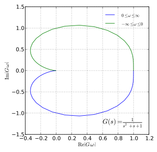
In control theory and stability theory, the Nyquist stability criterion or Strecker–Nyquist stability criterion, independently discovered by the German electrical engineer Felix Strecker at Siemens in 1930 and the Swedish-American electrical engineer Harry Nyquist at Bell Telephone Laboratories in 1932, is a graphical technique for determining the stability of a dynamical system.

The Nichols plot is a plot used in signal processing and control design, named after American engineer Nathaniel B. Nichols.

<span class="mw-page-title-main">Electronic filter topology</span> Electronic filter circuits defined by component connection

Electronic filter topology defines electronic filter circuits without taking note of the values of the components used but only the manner in which those components are connected.

Bode's sensitivity integral, discovered by Hendrik Wade Bode, is a formula that quantifies some of the limitations in feedback control of linear parameter invariant systems. Let L be the loop transfer function and S be the sensitivity function.

Iso-damping is a desirable system property referring to a state where the open-loop phase Bode plot is flat—i.e., the phase derivative with respect to the frequency is zero, at a given frequency called the "tangent frequency", $. At the "tangent frequency" the Nyquist curve of the open-loop system tangentially touches the sensitivity circle and the phase Bode is locally flat which implies that the system will be more robust to gain variations. For systems that exhibit iso-damping property, the overshoots of the closed-loop step responses will remain almost constant for different values of the controller gain. This will ensure that the closed-loop system is robust to gain variations.$

In control theory the Youla–Kučera parametrization is a formula that describes all possible stabilizing feedback controllers for a given plant P, as function of a single parameter Q.

Classical control theory is a branch of control theory that deals with the behavior of dynamical systems with inputs, and how their behavior is modified by feedback, using the Laplace transform as a basic tool to model such systems.

Data-driven control systems are a broad family of control systems, in which the identification of the process model and/or the design of the controller are based entirely on experimental data collected from the plant.

References

↑ K.J. Astrom, "Model uncertainty and robust control," in Lecture Notes on Iterative Identification and Control Design. Lund, Sweden: Lund Institute of Technology, Jan. 2000, pp. 63–100.
↑ K.J. Astrom and T. Hagglund, PID Controllers: Theory, Design and Tuning, 2nd ed. Research Triangle Park, NC 27709, USA: ISA - The Instrumentation, Systems, and Automation Society, 1995.
↑ A. G. Yepes, et al., "Analysis and design of resonant current controllers for voltage-source converters by means of Nyquist diagrams and sensitivity function" in IEEE Trans. on Industrial Electronics, vol. 58, No. 11, Nov. 2011, pp. 5231–5250.
↑ Karl Johan Åström and Richard M. Murray. Feedback systems : an introduction for scientists and engineers. Princeton University Press, Princeton, NJ, 2008.