


The sensitivity index or discriminability index or detectability index is a dimensionless statistic used in signal detection theory. A higher index indicates that the signal can be more readily detected.
The sensitivity index or discriminability index or detectability index is a dimensionless statistic used in signal detection theory. A higher index indicates that the signal can be more readily detected.
The discriminability index is the separation between the means of two distributions (typically the signal and the noise distributions), in units of the standard deviation.
For two univariate distributions and with the same standard deviation, it is denoted by ('dee-prime'):
In higher dimensions, i.e. with two multivariate distributions with the same variance-covariance matrix , (whose symmetric square-root, the standard deviation matrix, is ), this generalizes to the Mahalanobis distance between the two distributions:
where is the 1d slice of the sd along the unit vector through the means, i.e. the equals the along the 1d slice through the means. [1]
For two bivariate distributions with equal variance-covariance, this is given by:
where is the correlation coefficient, and here and , i.e. including the signs of the mean differences instead of the absolute. [1]
is also estimated as . [2] : 8
When the two distributions have different standard deviations (or in general dimensions, different covariance matrices), there exist several contending indices, all of which reduce to for equal variance/covariance.
This is the maximum (Bayes-optimal) discriminability index for two distributions, based on the amount of their overlap, i.e. the optimal (Bayes) error of classification by an ideal observer, or its complement, the optimal accuracy :
where is the inverse cumulative distribution function of the standard normal. The Bayes discriminability between univariate or multivariate normal distributions can be numerically computed [1] (Matlab code), and may also be used as an approximation when the distributions are close to normal.
is a positive-definite statistical distance measure that is free of assumptions about the distributions, like the Kullback-Leibler divergence . is asymmetric, whereas is symmetric for the two distributions. However, does not satisfy the triangle inequality, so it is not a full metric. [1]
In particular, for a yes/no task between two univariate normal distributions with means and variances , the Bayes-optimal classification accuracies are: [1]
where denotes the non-central chi-squared distribution, , and . The Bayes discriminability
can also be computed from the ROC curve of a yes/no task between two univariate normal distributions with a single shifting criterion. It can also be computed from the ROC curve of any two distributions (in any number of variables) with a shifting likelihood-ratio, by locating the point on the ROC curve that is farthest from the diagonal. [1]
For a two-interval task between these distributions, the optimal accuracy is ( denotes the generalized chi-squared distribution), where . [1] The Bayes discriminability .
A common approximate (i.e. sub-optimal) discriminability index that has a closed-form is to take the average of the variances, i.e. the rms of the two standard deviations: [3] (also denoted by ). It is times the -score of the area under the receiver operating characteristic curve (AUC) of a single-criterion observer. This index is extended to general dimensions as the Mahalanobis distance using the pooled covariance, i.e. with as the common sd matrix. [1]
Another index is , extended to general dimensions using as the common sd matrix. [1]
It has been shown that for two univariate normal distributions, , and for multivariate normal distributions, still. [1]
Thus, and underestimate the maximum discriminability of univariate normal distributions. can underestimate by a maximum of approximately 30%. At the limit of high discriminability for univariate normal distributions, converges to . These results often hold true in higher dimensions, but not always. [1] Simpson and Fitter [3] promoted as the best index, particularly for two-interval tasks, but Das and Geisler [1] have shown that is the optimal discriminability in all cases, and is often a better closed-form approximation than , even for two-interval tasks.
The approximate index , which uses the geometric mean of the sd's, is less than at small discriminability, but greater at large discriminability. [1]
In general, the contribution to the total discriminability by each dimension or feature may be measured using the amount by which the discriminability drops when that dimension is removed. If the total Bayes discriminability is and the Bayes discriminability with dimension removed is , we can define the contribution of dimension as . This is the same as the individual discriminability of dimension when the covariance matrices are equal and diagonal, but in the other cases, this measure more accurately reflects the contribution of a dimension than its individual discriminability. [1]

In physics, the Lorentz transformations are a six-parameter family of linear transformations from a coordinate frame in spacetime to another frame that moves at a constant velocity relative to the former. The respective inverse transformation is then parameterized by the negative of this velocity. The transformations are named after the Dutch physicist Hendrik Lorentz.
In probability theory, the central limit theorem (CLT) states that, under appropriate conditions, the distribution of a normalized version of the sample mean converges to a standard normal distribution. This holds even if the original variables themselves are not normally distributed. There are several versions of the CLT, each applying in the context of different conditions.

In probability theory and statistics, the multivariate normal distribution, multivariate Gaussian distribution, or joint normal distribution is a generalization of the one-dimensional (univariate) normal distribution to higher dimensions. One definition is that a random vector is said to be k-variate normally distributed if every linear combination of its k components has a univariate normal distribution. Its importance derives mainly from the multivariate central limit theorem. The multivariate normal distribution is often used to describe, at least approximately, any set of (possibly) correlated real-valued random variables each of which clusters around a mean value.

In probability theory and statistics, a covariance matrix is a square matrix giving the covariance between each pair of elements of a given random vector.
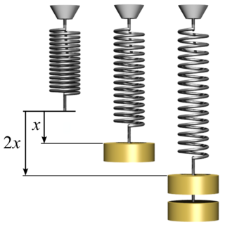
In physics, Hooke's law is an empirical law which states that the force needed to extend or compress a spring by some distance scales linearly with respect to that distance—that is, Fs = kx, where k is a constant factor characteristic of the spring, and x is small compared to the total possible deformation of the spring. The law is named after 17th-century British physicist Robert Hooke. He first stated the law in 1676 as a Latin anagram. He published the solution of his anagram in 1678 as: ut tensio, sic vis. Hooke states in the 1678 work that he was aware of the law since 1660.

In physics and mathematics, the Lorentz group is the group of all Lorentz transformations of Minkowski spacetime, the classical and quantum setting for all (non-gravitational) physical phenomena. The Lorentz group is named for the Dutch physicist Hendrik Lorentz.
Linear elasticity is a mathematical model of how solid objects deform and become internally stressed due to prescribed loading conditions. It is a simplification of the more general nonlinear theory of elasticity and a branch of continuum mechanics.
In statistics, propagation of uncertainty is the effect of variables' uncertainties on the uncertainty of a function based on them. When the variables are the values of experimental measurements they have uncertainties due to measurement limitations which propagate due to the combination of variables in the function.

In statistics, particularly in hypothesis testing, the Hotelling's T-squared distribution (T2), proposed by Harold Hotelling, is a multivariate probability distribution that is tightly related to the F-distribution and is most notable for arising as the distribution of a set of sample statistics that are natural generalizations of the statistics underlying the Student's t-distribution. The Hotelling's t-squared statistic (t2) is a generalization of Student's t-statistic that is used in multivariate hypothesis testing.
In differential geometry, the four-gradient is the four-vector analogue of the gradient from vector calculus.

The Maxwell stress tensor is a symmetric second-order tensor used in classical electromagnetism to represent the interaction between electromagnetic forces and mechanical momentum. In simple situations, such as a point charge moving freely in a homogeneous magnetic field, it is easy to calculate the forces on the charge from the Lorentz force law. When the situation becomes more complicated, this ordinary procedure can become impractically difficult, with equations spanning multiple lines. It is therefore convenient to collect many of these terms in the Maxwell stress tensor, and to use tensor arithmetic to find the answer to the problem at hand.
Bayesian linear regression is a type of conditional modeling in which the mean of one variable is described by a linear combination of other variables, with the goal of obtaining the posterior probability of the regression coefficients and ultimately allowing the out-of-sample prediction of the regressandconditional on observed values of the regressors. The simplest and most widely used version of this model is the normal linear model, in which given is distributed Gaussian. In this model, and under a particular choice of prior probabilities for the parameters—so-called conjugate priors—the posterior can be found analytically. With more arbitrarily chosen priors, the posteriors generally have to be approximated.
In statistics, the multivariate t-distribution is a multivariate probability distribution. It is a generalization to random vectors of the Student's t-distribution, which is a distribution applicable to univariate random variables. While the case of a random matrix could be treated within this structure, the matrix t-distribution is distinct and makes particular use of the matrix structure.
In probability and statistics, the class of exponential dispersion models (EDM), also called exponential dispersion family (EDF), is a set of probability distributions that represents a generalisation of the natural exponential family. Exponential dispersion models play an important role in statistical theory, in particular in generalized linear models because they have a special structure which enables deductions to be made about appropriate statistical inference.

In probability theory and statistics, the normal-inverse-gamma distribution is a four-parameter family of multivariate continuous probability distributions. It is the conjugate prior of a normal distribution with unknown mean and variance.
In probability theory and statistics, the negative multinomial distribution is a generalization of the negative binomial distribution (NB(x0, p)) to more than two outcomes.

In probability theory, a logit-normal distribution is a probability distribution of a random variable whose logit has a normal distribution. If Y is a random variable with a normal distribution, and t is the standard logistic function, then X = t(Y) has a logit-normal distribution; likewise, if X is logit-normally distributed, then Y = logit(X)= log (X/(1-X)) is normally distributed. It is also known as the logistic normal distribution, which often refers to a multinomial logit version (e.g.).
In probability theory and statistics, the normal-inverse-Wishart distribution is a multivariate four-parameter family of continuous probability distributions. It is the conjugate prior of a multivariate normal distribution with unknown mean and covariance matrix.
Lagrangian field theory is a formalism in classical field theory. It is the field-theoretic analogue of Lagrangian mechanics. Lagrangian mechanics is used to analyze the motion of a system of discrete particles each with a finite number of degrees of freedom. Lagrangian field theory applies to continua and fields, which have an infinite number of degrees of freedom.
In the mathematical theory of probability, multivariate Laplace distributions are extensions of the Laplace distribution and the asymmetric Laplace distribution to multiple variables. The marginal distributions of symmetric multivariate Laplace distribution variables are Laplace distributions. The marginal distributions of asymmetric multivariate Laplace distribution variables are asymmetric Laplace distributions.
| | This signal processing-related article is a stub. You can help Wikipedia by expanding it. |
| | This statistics-related article is a stub. You can help Wikipedia by expanding it. |


