
The Navier–Stokes equations are partial differential equations which describe the motion of viscous fluid substances. They were named after French engineer and physicist Claude-Louis Navier and the Irish physicist and mathematician George Gabriel Stokes. They were developed over several decades of progressively building the theories, from 1822 (Navier) to 1842–1850 (Stokes).
In mathematics and applied mathematics, perturbation theory comprises methods for finding an approximate solution to a problem, by starting from the exact solution of a related, simpler problem. A critical feature of the technique is a middle step that breaks the problem into "solvable" and "perturbative" parts. In perturbation theory, the solution is expressed as a power series in a small parameter . The first term is the known solution to the solvable problem. Successive terms in the series at higher powers of usually become smaller. An approximate 'perturbation solution' is obtained by truncating the series, usually by keeping only the first two terms, the solution to the known problem and the 'first order' perturbation correction.

Noether's theorem states that every continuous symmetry of the action of a physical system with conservative forces has a corresponding conservation law. This is the first of two theorems proven by mathematician Emmy Noether in 1915 and published in 1918. The action of a physical system is the integral over time of a Lagrangian function, from which the system's behavior can be determined by the principle of least action. This theorem only applies to continuous and smooth symmetries of physical space.
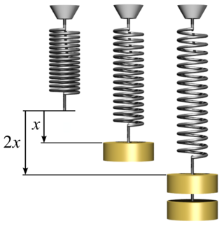
In physics, Hooke's law is an empirical law which states that the force needed to extend or compress a spring by some distance scales linearly with respect to that distance—that is, Fs = kx, where k is a constant factor characteristic of the spring, and x is small compared to the total possible deformation of the spring. The law is named after 17th-century British physicist Robert Hooke. He first stated the law in 1676 as a Latin anagram. He published the solution of his anagram in 1678 as: ut tensio, sic vis. Hooke states in the 1678 work that he was aware of the law since 1660.
Linear elasticity is a mathematical model of how solid objects deform and become internally stressed due to prescribed loading conditions. It is a simplification of the more general nonlinear theory of elasticity and a branch of continuum mechanics.

The phrase Yang–Mills theory means both a quantum field theory for nuclear binding devised by Chen Ning Yang and Robert Mills in 1953 and the class of similar theories. In mathematical physics, Yang–Mills theory is a gauge theory based on a special unitary group SU(n), or more generally any compact Lie group. A Yang–Mills theory seeks to describe the behavior of elementary particles using these non-abelian Lie groups and is at the core of the unification of the electromagnetic force and weak forces (i.e. U(1) × SU(2)) as well as quantum chromodynamics, the theory of the strong force (based on SU(3)). Thus it forms the basis of our understanding of the Standard Model of particle physics.
In quantum mechanics and quantum field theory, the propagator is a function that specifies the probability amplitude for a particle to travel from one place to another in a given period of time, or to travel with a certain energy and momentum. In Feynman diagrams, which serve to calculate the rate of collisions in quantum field theory, virtual particles contribute their propagator to the rate of the scattering event described by the respective diagram. These may also be viewed as the inverse of the wave operator appropriate to the particle, and are, therefore, often called (causal) Green's functions.
In statistics, a confidence region is a multi-dimensional generalization of a confidence interval. It is a set of points in an n-dimensional space, often represented as an ellipsoid around a point which is an estimated solution to a problem, although other shapes can occur.
In econometrics, endogeneity broadly refers to situations in which an explanatory variable is correlated with the error term. The distinction between endogenous and exogenous variables originated in simultaneous equations models, where one separates variables whose values are determined by the model from variables which are predetermined. Ignoring simultaneity in the estimation leads to biased estimates as it violates the exogeneity assumption of the Gauss–Markov theorem. The problem of endogeneity is often ignored by researchers conducting non-experimental research and doing so precludes making policy recommendations. Instrumental variable techniques are commonly used to mitigate this problem.
In mathematics, more specifically in dynamical systems, the method of averaging exploits systems containing time-scales separation: a fast oscillationversus a slow drift. It suggests that we perform an averaging over a given amount of time in order to iron out the fast oscillations and observe the qualitative behavior from the resulting dynamics. The approximated solution holds under finite time inversely proportional to the parameter denoting the slow time scale. It turns out to be a customary problem where there exists the trade off between how good is the approximated solution balanced by how much time it holds to be close to the original solution.
In mathematics, the method of matched asymptotic expansions is a common approach to finding an accurate approximation to the solution to an equation, or system of equations. It is particularly used when solving singularly perturbed differential equations. It involves finding several different approximate solutions, each of which is valid for part of the range of the independent variable, and then combining these different solutions together to give a single approximate solution that is valid for the whole range of values of the independent variable. In the Russian literature, these methods were known under the name of "intermediate asymptotics" and were introduced in the work of Yakov Zeldovich and Grigory Barenblatt.
In physics and fluid mechanics, a Blasius boundary layer describes the steady two-dimensional laminar boundary layer that forms on a semi-infinite plate which is held parallel to a constant unidirectional flow. Falkner and Skan later generalized Blasius' solution to wedge flow, i.e. flows in which the plate is not parallel to the flow.

In physics, Hamilton's principle is William Rowan Hamilton's formulation of the principle of stationary action. It states that the dynamics of a physical system are determined by a variational problem for a functional based on a single function, the Lagrangian, which may contain all physical information concerning the system and the forces acting on it. The variational problem is equivalent to and allows for the derivation of the differential equations of motion of the physical system. Although formulated originally for classical mechanics, Hamilton's principle also applies to classical fields such as the electromagnetic and gravitational fields, and plays an important role in quantum mechanics, quantum field theory and criticality theories.

A Belinski–Khalatnikov–Lifshitz (BKL) singularity is a model of the dynamic evolution of the universe near the initial gravitational singularity, described by an anisotropic, chaotic solution of the Einstein field equation of gravitation. According to this model, the universe is chaotically oscillating around a gravitational singularity in which time and space become equal to zero or, equivalently, the spacetime curvature becomes infinitely big. This singularity is physically real in the sense that it is a necessary property of the solution, and will appear also in the exact solution of those equations. The singularity is not artificially created by the assumptions and simplifications made by the other special solutions such as the Friedmann–Lemaître–Robertson–Walker, quasi-isotropic, and Kasner solutions.
The turbulent Prandtl number (Prt) is a non-dimensional term defined as the ratio between the momentum eddy diffusivity and the heat transfer eddy diffusivity. It is useful for solving the heat transfer problem of turbulent boundary layer flows. The simplest model for Prt is the Reynolds analogy, which yields a turbulent Prandtl number of 1. From experimental data, Prt has an average value of 0.85, but ranges from 0.7 to 0.9 depending on the Prandtl number of the fluid in question.

In numerical analysis, the interval finite element method is a finite element method that uses interval parameters. Interval FEM can be applied in situations where it is not possible to get reliable probabilistic characteristics of the structure. This is important in concrete structures, wood structures, geomechanics, composite structures, biomechanics and in many other areas. The goal of the Interval Finite Element is to find upper and lower bounds of different characteristics of the model and use these results in the design process. This is so called worst case design, which is closely related to the limit state design.

Anatoly Alexeyevich Karatsuba was a Russian mathematician working in the field of analytic number theory, p-adic numbers and Dirichlet series.
The Krylov–Bogolyubov averaging method is a mathematical method for approximate analysis of oscillating processes in non-linear mechanics. The method is based on the averaging principle when the exact differential equation of the motion is replaced by its averaged version. The method is named after Nikolay Krylov and Nikolay Bogoliubov.

The Kirchhoff–Love theory of plates is a two-dimensional mathematical model that is used to determine the stresses and deformations in thin plates subjected to forces and moments. This theory is an extension of Euler-Bernoulli beam theory and was developed in 1888 by Love using assumptions proposed by Kirchhoff. The theory assumes that a mid-surface plane can be used to represent a three-dimensional plate in two-dimensional form.
Phase reduction is a method used to reduce a multi-dimensional dynamical equation describing a nonlinear limit cycle oscillator into a one-dimensional phase equation. Many phenomena in our world such as chemical reactions, electric circuits, mechanical vibrations, cardiac cells, and spiking neurons are examples of rhythmic phenomena, and can be considered as nonlinear limit cycle oscillators.


