Strict Fibonacci heap

Last updated
Strict Fibonacci heap
Type Heap
Invented2012
Invented byGerth S. Brodal, George Lagogiannis, and Robert E. Tarjan
Complexities in big O notation
Space complexity
Space O(n)
Time complexity
Function Amortized Worst Case
Insert O(1)
Find-min O(1)
Delete-min O(log n)
Decrease-key O(1)
Merge O(1)

In computer science, a strict Fibonacci heap is a priority queue data structure with low worst case time bounds. It matches the amortized time bounds of the Fibonacci heap in the worst case. To achieve these time bounds, strict Fibonacci heaps maintain several invariants by performing restoring transformations after every operation. These transformations can be done in constant time by using auxiliary data structures to track invariant violations, and the pigeonhole principle guarantees that these can be fixed. Strict Fibonacci heaps were invented in 2012 by Gerth S. Brodal, George Lagogiannis, and Robert E. Tarjan.

Contents

Along with Brodal queues, strict Fibonacci heaps belong to a class of asymptotically optimal data structures for priority queues. [1] All operations on strict Fibonacci heaps run in worst case constant time except delete-min, which is necessarily logarithmic. This is optimal, because any priority queue can be used to sort a list of elements by performing insertions and delete-min operations. [2] However, strict Fibonacci heaps are simpler than Brodal queues, which make use of dynamic arrays and redundant counters, [3] whereas the strict Fibonacci heap is pointer based only.

Structure

A strict Fibonacci heap with no loss. Nodes 5 and 2 are active roots. Their active subtrees are binomial trees. 12 node strict Fibonacci Heap.png
A strict Fibonacci heap with no loss. Nodes 5 and 2 are active roots. Their active subtrees are binomial trees.

A strict Fibonacci heap is a single tree satisfying the minimum-heap property. That is, the key of a node is always smaller than or equal to its children. As a direct consequence, the node with the minimum key always lies at the root.

Like ordinary Fibonacci heaps, [4] strict Fibonacci heaps possess substructures similar to binomial heaps. To identify these structures, we label every node with one of two types. We thus introduce the following definitions and rules:

Invariants

Invariant 1: Structure
The th rightmost active child of an active node satisfies .

Thus, the loss of an active node can be viewed as a generalisation of Fibonacci heap 'marks'. For example, a subtree consisting of only active nodes with loss zero is a binomial tree.

In addition, several invariants which impose logarithmic bounds on three main quantities: the number of active roots, the total loss, and the degrees of nodes. This is in contrast to the ordinary Fibonacci heap, which is more flexible and allows structural violations to grow on the order of to be cleaned up later, as it is a lazy data structure.

To assists in keeping the degrees of nodes logarithmic, every non-root node also participates in a queue . In the following section, and for rest of this article, we define the real number , where is the number of nodes in the heap, and denotes the binary logarithm.

Invariant 2: Active roots
The total number of active roots is at most .
Invariant 3: Total loss
The total loss in the heap is at most .
Invariant 4: Root degree
The degree of the root is at most .
Invariant 5: Non-root degrees
For an active node with zero loss, the degree is at most , where is its position in (with 1 as the first element). For all other non-root nodes, the degree is at most .
Corollary 1: Maximum degree
The degree of any non-root node is at most .
Proof:
This follows immediately from invariant 5. Letting , we have
Lemma 1: Maximum rank
If invariant 1 holds, the maximum rank or any active node is at most , where is the total loss. [5]
Proof:
We proceed by contradiction. Let be an active node with maximal rank in a heap with nodes and total loss , and assume that , where is the smallest integer such that . Our goal is to show that the subtree rooted at contains nodes, which is a contradiction because there are only nodes in the heap.
Discard all subtrees rooted at passive nodes from , leaving it with only active nodes. Cut off all the grandchildren of whose subtrees contain any node of positive loss, and increase the loss of the children of accordingly, once for each grandchild lost. The quantity is unchanged for the remaining nodes, preserving invariant 1. Furthermore, the total loss is still at most .
The children of now consists of loss-free subtrees and leaf nodes with positive loss. Currently, satisfies for the th rightmost child of . We make this an exact equality by first reducing the loss of each , and pruning any grandchildren if necessary. Afterwards, exactly. All other descendants of are also converted into binomial subtrees by pruning children as necessary.
We now attempt to reconstruct a minimal version of by starting with a binomial tree of degree , containing active nodes. We wish to increase the loss to , but keep the rank of as and the number of nodes as low as possible. For a binomial tree of degree , there is one child of each degree from to . Hence, there are grandchildren of order . If we cut all the grandchildren whose degree , then we have cut grandchildren, which is sufficient to bring the loss up to . All grandchildren with degree survive. Let be the child of with degree and loss 0. By assumption, , and is a complete binomial tree, so it has at least nodes. Since this would mean has at least nodes, we have reached a contradiction, and therefore . Noting that , we obtain .
Corollary 2: Maximum rank
If invariants 1 and 3 both hold, then the maximum rank is .
Proof:
From invariant 3, we have . By substituting this into lemma 1, we calculate as follows:

Transformations

The following transformations restore the above invariants after a priority queue operation has been performed. There are three main quantities we wish to minimize: the number of active roots, the total loss in the heap, and the degree of the root. All transformations can be performed in time, which is possible by maintaining auxiliary data structures to track candidate nodes (described in the section on implementation). [5]

Active root reduction

Let and be active roots with equal rank , and assume . Link as the leftmost child of and increase the rank of by 1. If the rightmost child of is passive, link to the root.

As a result, is no longer an active root, so the number of active roots decreases by 1. However, the degree of the root node may increase by 1,

Since becomes the th rightmost child of , and has rank , invariant 1 is preserved.

Lemma 2: Availability of active root reduction
If invariant 2 is violated, but invariants 1 and 3 hold, then active root reduction is possible.
Proof:
Because invariant 2 is broken, there are more than active roots present. From corollary 2, the maximum rank of a node is . By the pigeonhole principle, there exists a pair of active roots with the same rank.

Loss reduction

One node loss reduction

Let be an active non-root with loss at least 2. Link to the root, thus turning it into an active root, and resetting its loss to 0. Let the original parent of be . must be active, since otherwise would have previously been an active root, and thus could not have had positive loss. The rank of is decreased by 1. If is not an active root, increase its loss by 1.

Overall, the total loss decreases by 1 or 2. As a side effect, the root degree and number of active roots increase by 1, making it less preferable to two node loss reduction, but still a necessary operation.

Two node loss reduction

Let  and  be active nodes with equal rank  and loss equal to 1, and let be the parent of . Without loss of generality, assume that . Detach from , and link to . Increase the rank of by 1 and reset the loss of and from 1 to 0.

must be active, since had positive loss and could not have been an active root. Hence, the rank of is decreased by 1. If is not an active root, increase its loss by 1.

Overall, the total loss decreases by either 1 or 2, with no side effects.

Lemma 3: Availability of loss reduction
If invariant 3 is violated by 1, but invariant 2 holds, then loss reduction is possible.
Proof: We apply the pigeonhole principle again. If invariant 3 is violated by 1, the total loss is . Lemma 1 can be reformulated to also work with . Thus, corollary 2 holds. Since the maximum rank is , either there either exists a pair of active nodes with equal rank and loss 1, or an active node with . Both cases present an opportunity for loss reduction.

Root degree reduction

Root degree reduction Strict Fibonacci heap root degree reduction.svg
Root degree reduction

Let , , and be the three rightmost passive linkable children of the root. Detach them all from the root and sort them such that . Change and to be active. Link to , link to , and link as the leftmost child of the root. As a result, becomes an active root with rank 1 and loss 0. The rank and loss of is set to 0.

The net change of this transformation is that the degree of the root node decreases by 2. As a side effect, the number of active roots increases by 1.

Lemma 4: Availability of root degree reduction
If invariant 4 is violated, but invariant 2 holds, then root degree reduction is possible.
Proof:
If invariant 4 is broken, then the degree of the root is at least . The children of the root fall into three categories: active roots, passive non-linkable nodes, and passive linkable nodes. Each passive non-linkable node subsumes an active root, since its subtree contains at least one active node. Because the number of active roots is at most , the rightmost three children of the root must therefore be passive linkable.

Summary

The following table summarises the effect of each transformation on the three important quantities. Individually, each transformation may violate invariants, but we are only interested in certain combinations of transformations which do not increase any of these quantities.

Effect of transformations
Active rootsTotal lossRoot degree
Active root reduction
Root degree reduction
One node loss reduction
Two node loss reduction

When deciding which transformations to perform, we consider only the worst case effect of these operations, for simplicity. The two types of loss reduction are also considered to be the same operation. As such, we define 'performing a loss reduction' to mean attempting each type of loss reduction in turn.

Worst case effect of transformations
Active rootsTotal lossRoot degree
Active root reduction
Root degree reduction
Loss reduction

Implementation

Linking nodes

To ensure active nodes lie to the left of passive nodes, and preserve invariant 1, the linking operation should place active nodes on the left, and passive nodes on the right. It is necessary for active and passive nodes to coexist in the same list, because the merge operation changes all nodes in the smaller heap to be passive. If they existed in two separate lists, the lists would have to be concatenated, which cannot be done in constant time for all nodes.

For the root, we also pose the requirement that passive linkable children lie to the right of the passive non-linkable children. Since we wish to be able link nodes to the root in constant time, a pointer to the first passive linkable child of the root must be maintained.

Finding candidate nodes

The invariant restoring transformations rely on being able to find candidate nodes in time. This means that we must keep track of active roots with the same rank, nodes with loss 1 of the same rank, and nodes with loss at least 2.

The original paper by Brodal et al. described a fix-list and a rank-list as a way of tracking candidate nodes. [5]

Fix-list

Rank-list and fix-list Rank-list and fix-list in Strict Fibonacci heap.svg
Rank-list and fix-list

The fix-list is divided into four parts:

  1. Active roots ready for active root reduction – active roots with a partner of the same rank. Nodes with the same rank are kept adjacent.
  2. Active roots not yet ready for active reduction – the only active roots for that rank.
  3. Active nodes with loss 1 that are not yet ready for loss reduction – the only active nodes with loss 1 for that rank.
  4. Active nodes that are ready for loss reduction – This includes active nodes with loss 1 that have a partner of the same rank, and active nodes with loss at least 2, which do not need partners to be reduced. Nodes with the same rank are kept adjacent.

To check if active root reduction is possible, we simply check if part 1 is non-empty. If it is non-empty, the first two nodes can be popped off and transformed. Similarly, to check if loss reduction is possible, we check the end of part 4. If it contains a node with loss at least 2, one node loss reduction is performed. Otherwise, if the last two nodes both have loss 1, and are of the same rank, two node loss reduction is performed.

Rank-list

The rank-list is a doubly linked list containing information about each rank, to allow nodes of the same rank to be partnered together in the fix-list.

For each node representing rank in the rank-list, we maintain:

  • A pointer to the first active root in the fix-list with rank . If such a node does not exist, this is NULL.
  • A pointer to the first active node in the fix-list with rank and loss 1. If such a node does not exist, this is NULL.
  • A pointer to the node representing rank and , to facilitate the incrementation and decrementation of ranks.

The fix-list and rank-list require extensive bookkeeping, which must be done whenever a new active node arises, or when the rank or loss of a node is changed.

Shared flag

Using a shared flag to change make all nodes passive in
O
(
1
)
{\displaystyle O(1)}
time Shared-pointers.svg
Using a shared flag to change make all nodes passive in time

The merge operation changes all of the active nodes of the smaller heap into passive nodes. This can be done in time by introducing a level of indirection. [5] Instead of a boolean flag, each active node has a pointer towards an active flag object containing a boolean value. For passive nodes, it does not matter which active flag object they point to, as long as the flag object is set to passive, because it is not required to change many passive nodes into active nodes simultaneously.

Relinking pointers between nodes and boxed keys Strict Fibonacci heap boxed keys.svg
Relinking pointers between nodes and boxed keys

Storing keys

The decrease-key operation requires a reference to the node we wish to decrease the key of. However, the decrease-key operation itself sometimes swaps the key of a node and the key root.

Assume that the insert operation returns some opaque reference that we can call decrease-key on, as part of the public API. If these references are internal heap nodes, then by swapping keys we have mutated these references, causing other references to become undefined. To ensure a key is always stays with the same reference, it is necessary to 'box' the key. Each heap node now contains a pointer to a box containing a key, and the box also has a pointer to the heap node. When inserting an item, we create a box to store the key in, link the heap node to the box both ways, and return the box object. [5] To swap the keys between two nodes, we re-link the pointers between the boxes and nodes instead.

Operations

Merge

Let and be strict Fibonacci heaps. If either is empty, return the other. Otherwise, let and be their corresponding sizes. Without loss of generality, assume that . Since the sizes of the fix-list and rank-list of each heap are logarithmic with respect to the heap size, it is not possible to merge these auxiliary structures in constant time. Instead, we throw away the structure of the smaller heap by discarding its fix-list and rank-list, and converting all of its nodes into passive nodes. [5] This can be done in constant time, using a shared flag, as shown above. Link and , letting the root with the smaller key become the parent of the other. Let and be the queues of and respectively. The queue of resulting heap is set to, where is the root with the larger key.

The only possible structural violation is the root degree. This is solved by performing 1 active root reduction, and 1 root degree reduction, if each transformation is possible.

Active rootsTotal lossRoot degree
State after merge
Active root reduction
Root degree reduction
Total

Proof of correctness

Invariants 1, 2, and 3 hold automatically, since the structure of the heap is discarded. As calculated above, any violations of invariant 4 are solved by the root degree reduction transformation.

To verify invariant 5, we consider the final positions of nodes in . Each node has its degree bounded by or .

For the smaller heap the positions in are unchanged. However, all nodes in are now passive, which means that their constraint may change from the case to the case. But noting that , the resulting size is at least double . This results in an increase of at least 1 on each constraint, which eliminates the previous concern.

The root with the larger key between and becomes a non-root, and is placed between and at position . By invariant 4, its degree was bounded by either or , depending on which heap it came from. It is easy to see that this is less than in any case.

For the larger heap, the positions increase by . But since the resulting size is , the value actually increases, weakening the constraint.

Insert

Insertion can be considered a special case of the merge operation. To insert a single key, create a new heap containing a single passive node and an empty queue, and merge it with the main heap.

Find-min

Due to the minimum-heap property, the node with the minimum key is always at the root, if it exists.

Delete-min

Delete-min operation Strict Fibonacci heap delete-min.svg
Delete-min operation

If the root is the only node in the heap, we are done by simply removing it. Otherwise, search the children of the root to find the node with minimum key, and set the new root to . If is active, make it passive, causing all active children of to implicitly become active roots. Link the children of the old root to . Since is now the root, move all of its passive linkable children to the right, and remove from .

The degree of the root approximately doubles, because we have linked all the children of the old root to . We perform the following restorative transformations:

  1. Repeat twice: rotate by moving the head of to the back, and link the two rightmost passive children of to the root.
  2. If a loss reduction is possible, perform it.
  3. Perform active root reductions and root degree reductions until neither is possible.

To see how step 3 is bounded, consider the state after step 3:

Active rootsTotal lossRoot degree
State after delete-min
Queue rotation
Loss reduction
Total

Observe that, 3 active root reductions and 2 root reductions decreases the root degree and active roots by 1:

Active rootsTotal lossRoot degree
Active root reduction
Root degree reduction
Total

Since , step 3 never executes more than times.

Proof of correctness

Invariant 1 holds trivially, since no active roots are created.

The size of the heap decreases by one, causing decreases by at most one. Thus, invariant 3 is violated by at most 1. By lemma 3, loss reduction is possible, which has been done by step 2.

Invariants 1 and 3 now hold. If invariants 2 and 4 were still violated after step 3, it would be possible to apply active root reduction and root degree reduction, by lemmas 2 and 4. However, active root reduction and root degree reduction have already been exhaustively applied. Therefore, invariants 2 and 4 also hold.

To show that invariant 5 is satisfied, we first note that the heap size has decreased by 1. Because the first 2 nodes in are popped in step 1, the positions of the other elements in decrease by 2. Therefore, the degree constraints and remain constant for these nodes. The two nodes which were popped previously had positions 1 and 2 in , and now have positions and respectively. The effect is that their degree constraints have strengthed by 2, however, we cut off two passive children for each of these nodes, which is sufficient to satisfy the constraint again.

Decrease-key

Decrease-key operation Sfh decrease key 1.svg
Decrease-key operation

Let be the node whose key has been decreased. If is the root, we are done. Otherwise, detach the subtree rooted at , and link it to the root. If the key of is smaller than the key of the root, swap their keys.

Up to three structural violations may have occurred. Unless was already a child of the root, the degree of the root increases by 1. When was detached from its original parent , we have the following cases:

In the worst case, all three quantities (root degree, total loss, active roots) increase by 1.

After performing 1 loss reduction, the worst case result is still that the root degree and number of active roots have both increased by 2. To fix these violations, we use the fact that 3 active root reductions and 2 root reductions decrease both of these quantities by 1. Hence, applying these transformations 6 and 4 times respectively is sufficient to eliminate all violations.

Active rootsTotal lossRoot degree
State after decrease-key
Loss reduction
Active root reduction
Root degree reduction
Total

Proof of correctness

The nodes which were previously the left siblings of move to fill the gap left by , decreasing their index. Since their constraint has weakened, invariant 1 is unaffected. Invariant 5 trivially holds as is unchanged.

Lemmas 2, 3 and 4 guarantee the availability of active root reduction, loss reduction, and root degree reduction. Therefore, invariants 2, 3 and 4 hold.

Performance

Although theoretically optimal, strict Fibonacci heaps are not useful in practical applications. They are extremely complicated to implement, requiring management of more than 10 pointers per node. [5] [6] While most operations run in time, the constant factors may be very high, making them up to 20 times slower than their more common counterparts such as binary heaps or pairing heaps. [7] Despite being relatively simpler, experiments show that in practice the strict Fibonacci heap performs slower than the Brodal queue. [8]

Summary of running times

Here are time complexities [9] of various heap data structures. Function names assume a min-heap. For the meaning of "O(f)" and "Θ(f)" see Big O notation.

Operationfind-mindelete-mininsertdecrease-keymeld
Binary [9] Θ(1)Θ(log n)O(log n)O(log n)Θ(n)
Leftist Θ(1)Θ(log n)Θ(log n)O(log n)Θ(log n)
Binomial [9] [10] Θ(1)Θ(log n)Θ(1) [lower-alpha 1] Θ(log n)O(log n)
Skew binomial [11] Θ(1)Θ(log n)Θ(1)Θ(log n)O(log n) [lower-alpha 2]
Pairing [12] Θ(1)O(log n) [lower-alpha 1] Θ(1)o(log n) [lower-alpha 1] [lower-alpha 3] Θ(1)
Rank-pairing [15] Θ(1)O(log n) [lower-alpha 1] Θ(1)Θ(1) [lower-alpha 1] Θ(1)
Fibonacci [9] [16] Θ(1)O(log n) [lower-alpha 1] Θ(1)Θ(1) [lower-alpha 1] Θ(1)
Strict Fibonacci [17] Θ(1)O(log n)Θ(1)Θ(1)Θ(1)
Brodal [18] [lower-alpha 4] Θ(1)O(log n)Θ(1)Θ(1)Θ(1)
2–3 heap [20] Θ(1)O(log n) [lower-alpha 1] Θ(1) [lower-alpha 1] Θ(1)?
  1. 1 2 3 4 5 6 7 8 9 Amortized time.
  2. Brodal and Okasaki describe a technique to reduce the worst-case complexity of meld to Θ(1); this technique applies to any heap datastructure that has insert in Θ(1) and find-min, delete-min, meld in O(log n).
  3. Lower bound of [13] upper bound of [14]
  4. Brodal and Okasaki later describe a persistent variant with the same bounds except for decrease-key, which is not supported. Heaps with n elements can be constructed bottom-up in O(n). [19]

Related Research Articles

<span class="mw-page-title-main">Heap (data structure)</span> Computer science data structure

In computer science, a heap is a tree-based data structure that satisfies the heap property: In a max heap, for any given node C, if P is a parent node of C, then the key of P is greater than or equal to the key of C. In a min heap, the key of P is less than or equal to the key of C. The node at the "top" of the heap is called the root node.

In computer science, a priority queue is an abstract data-type similar to a regular queue or stack data structure. Each element in a priority queue has an associated priority. In a priority queue, elements with high priority are served before elements with low priority. In some implementations, if two elements have the same priority, they are served in the same order in which they were enqueued. In other implementations, the order of elements with the same priority is undefined.

A splay tree is a binary search tree with the additional property that recently accessed elements are quick to access again. Like self-balancing binary search trees, a splay tree performs basic operations such as insertion, look-up and removal in O(log n) amortized time. For random access patterns drawn from a non-uniform random distribution, their amortized time can be faster than logarithmic, proportional to the entropy of the access pattern. For many patterns of non-random operations, also, splay trees can take better than logarithmic time, without requiring advance knowledge of the pattern. According to the unproven dynamic optimality conjecture, their performance on all access patterns is within a constant factor of the best possible performance that could be achieved by any other self-adjusting binary search tree, even one selected to fit that pattern. The splay tree was invented by Daniel Sleator and Robert Tarjan in 1985.

<span class="mw-page-title-main">Dijkstra's algorithm</span> Algorithm for finding shortest paths

Dijkstra's algorithm is an algorithm for finding the shortest paths between nodes in a weighted graph, which may represent, for example, road networks. It was conceived by computer scientist Edsger W. Dijkstra in 1956 and published three years later.

<span class="mw-page-title-main">Binary heap</span> Variant of heap data structure

A binary heap is a heap data structure that takes the form of a binary tree. Binary heaps are a common way of implementing priority queues. The binary heap was introduced by J. W. J. Williams in 1964, as a data structure for heapsort.

In computer science, a binomial heap is a data structure that acts as a priority queue. It is an example of a mergeable heap, as it supports merging two heaps in logarithmic time. It is implemented as a heap similar to a binary heap but using a special tree structure that is different from the complete binary trees used by binary heaps. Binomial heaps were invented in 1978 by Jean Vuillemin.

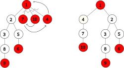
In computer science, a Fibonacci heap is a data structure for priority queue operations. It has a better amortized running time than many other priority queue data structures including the binary heap and binomial heap. consisting of a collection of heap-ordered trees. Michael L. Fredman and Robert E. Tarjan developed Fibonacci heaps in 1984 and published them in a scientific journal in 1987. Fibonacci heaps are named after the Fibonacci numbers, which are used in their running time analysis.

In mathematics, an algebraic torus, where a one dimensional torus is typically denoted by , , or , is a type of commutative affine algebraic group commonly found in projective algebraic geometry and toric geometry. Higher dimensional algebraic tori can be modelled as a product of algebraic groups . These groups were named by analogy with the theory of tori in Lie group theory. For example, over the complex numbers the algebraic torus is isomorphic to the group scheme , which is the scheme theoretic analogue of the Lie group . In fact, any -action on a complex vector space can be pulled back to a -action from the inclusion as real manifolds.

In computer science, a 2–3 heap is a data structure, a variation on the heap, designed by Tadao Takaoka in 1999. The structure is similar to the Fibonacci heap, and borrows from the 2–3 tree.

<span class="mw-page-title-main">AC power</span> Power in alternating current systems

In an electric circuit, instantaneous power is the time rate of flow of energy past a given point of the circuit. In alternating current circuits, energy storage elements such as inductors and capacitors may result in periodic reversals of the direction of energy flow. Its SI unit is the watt.

In information theory and machine learning, information gain is a synonym for Kullback–Leibler divergence; the amount of information gained about a random variable or signal from observing another random variable. However, in the context of decision trees, the term is sometimes used synonymously with mutual information, which is the conditional expected value of the Kullback–Leibler divergence of the univariate probability distribution of one variable from the conditional distribution of this variable given the other one.

In computer science, a leftist tree or leftist heap is a priority queue implemented with a variant of a binary heap. Every node x has an s-value which is the distance to the nearest leaf in subtree rooted at x. In contrast to a binary heap, a leftist tree attempts to be very unbalanced. In addition to the heap property, leftist trees are maintained so the right descendant of each node has the lower s-value.

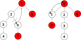
A pairing heap is a type of heap data structure with relatively simple implementation and excellent practical amortized performance, introduced by Michael Fredman, Robert Sedgewick, Daniel Sleator, and Robert Tarjan in 1986. Pairing heaps are heap-ordered multiway tree structures, and can be considered simplified Fibonacci heaps. They are considered a "robust choice" for implementing such algorithms as Prim's MST algorithm, and support the following operations :

In mathematics, the spin representations are particular projective representations of the orthogonal or special orthogonal groups in arbitrary dimension and signature. More precisely, they are two equivalent representations of the spin groups, which are double covers of the special orthogonal groups. They are usually studied over the real or complex numbers, but they can be defined over other fields.

<span class="mw-page-title-main">Cartesian tree</span> Binary tree derived from a sequence of numbers

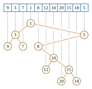
In computer science, a Cartesian tree is a binary tree derived from a sequence of distinct numbers. To construct the Cartesian tree, set its root to be the minimum number in the sequence, and recursively construct its left and right subtrees from the subsequences before and after this number. It is uniquely defined as a min-heap whose symmetric (in-order) traversal returns the original sequence.

In the study of denotational semantics of the lambda calculus, Böhm trees, Lévy-Longo trees, and Berarducci trees are tree-like mathematical objects that capture the "meaning" of a term up to some set of "meaningless" terms.

In computer science, a min-max heap is a complete binary tree data structure which combines the usefulness of both a min-heap and a max-heap, that is, it provides constant time retrieval and logarithmic time removal of both the minimum and maximum elements in it. This makes the min-max heap a very useful data structure to implement a double-ended priority queue. Like binary min-heaps and max-heaps, min-max heaps support logarithmic insertion and deletion and can be built in linear time. Min-max heaps are often represented implicitly in an array; hence it's referred to as an implicit data structure.

In computer science, a skew binomial heap is a data structure for priority queue operations. It is a variant of the binomial heap that supports constant-time insertion operations in the worst case, rather than amortized time.

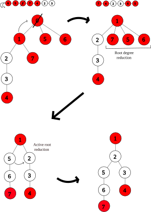
In computer science, the Brodal queue is a heap/priority queue structure with very low worst case time bounds: for insertion, find-minimum, meld and decrease-key and for delete-minimum and general deletion. They are the first heap variant to achieve these bounds without resorting to amortization of operational costs. Brodal queues are named after their inventor Gerth Stølting Brodal.

In graph theory, Yen's algorithm computes single-source K-shortest loopless paths for a graph with non-negative edge cost. The algorithm was published by Jin Y. Yen in 1971 and employs any shortest path algorithm to find the best path, then proceeds to find K − 1 deviations of the best path.

References

  1. Brodal, Gerth Stølting; Okasaki, Chris (November 1996). "Optimal purely functional priority queues". Journal of Functional Programming. 6 (6): 839–857. doi:10.1017/S095679680000201X. ISSN   0956-7968.
  2. Knuth, Donald E. (1998-04-24). The Art of Computer Programming: Sorting and Searching, Volume 3. Addison-Wesley Professional. ISBN   978-0-321-63578-5.
  3. Brodal, Gerth Stølting (1996-01-28). "Worst-case efficient priority queues". Proceedings of the Seventh Annual ACM-SIAM Symposium on Discrete Algorithms. SODA '96. USA: Society for Industrial and Applied Mathematics: 52–58. ISBN   978-0-89871-366-4.
  4. Fredman, Michael L.; Tarjan, Robert Endre (1987-07-01). "Fibonacci heaps and their uses in improved network optimization algorithms". Journal of the ACM. 34 (3): 596–615. doi:10.1145/28869.28874. ISSN   0004-5411.
  5. 1 2 3 4 5 6 7 Brodal, Gerth Stølting; Lagogiannis, George; Tarjan, Robert E. (2012-05-19). "Strict fibonacci heaps". Proceedings of the forty-fourth annual ACM symposium on Theory of computing. STOC '12. New York, NY, USA: Association for Computing Machinery. pp. 1177–1184. doi:10.1145/2213977.2214082. ISBN   978-1-4503-1245-5.
  6. Majerech, Vladan (2019-11-25), Fast Fibonacci heaps with worst case extensions, arXiv: 1911.11637
  7. Larkin, Daniel; Sen, Siddhartha; Tarjan, Robert (2014). "A Back-to-Basics Empirical Study of Priority Queues". Proceedings of the Sixteenth Workshop on Algorithm Engineering and Experiments: 61–72. arXiv: 1403.0252 . Bibcode:2014arXiv1403.0252L. doi:10.1137/1.9781611973198.7. ISBN   978-1-61197-319-8. S2CID   15216766.
  8. Mrena, Michal; Sedlacek, Peter; Kvassay, Miroslav (June 2019). "Practical Applicability of Advanced Implementations of Priority Queues in Finding Shortest Paths". 2019 International Conference on Information and Digital Technologies (IDT). Zilina, Slovakia: IEEE. pp. 335–344. doi:10.1109/DT.2019.8813457. ISBN   9781728114019. S2CID   201812705.
  9. 1 2 3 4 Cormen, Thomas H.; Leiserson, Charles E.; Rivest, Ronald L. (1990). Introduction to Algorithms (1st ed.). MIT Press and McGraw-Hill. ISBN   0-262-03141-8.
  10. "Binomial Heap | Brilliant Math & Science Wiki". brilliant.org. Retrieved 2019-09-30.
  11. Brodal, Gerth Stølting; Okasaki, Chris (November 1996), "Optimal purely functional priority queues", Journal of Functional Programming, 6 (6): 839–857, doi: 10.1017/s095679680000201x
  12. Iacono, John (2000), "Improved upper bounds for pairing heaps", Proc. 7th Scandinavian Workshop on Algorithm Theory (PDF), Lecture Notes in Computer Science, vol. 1851, Springer-Verlag, pp. 63–77, arXiv: 1110.4428 , CiteSeerX   10.1.1.748.7812 , doi:10.1007/3-540-44985-X_5, ISBN   3-540-67690-2
  13. Fredman, Michael Lawrence (July 1999). "On the Efficiency of Pairing Heaps and Related Data Structures" (PDF). Journal of the Association for Computing Machinery . 46 (4): 473–501. doi:10.1145/320211.320214.
  14. Pettie, Seth (2005). Towards a Final Analysis of Pairing Heaps (PDF). FOCS '05 Proceedings of the 46th Annual IEEE Symposium on Foundations of Computer Science. pp. 174–183. CiteSeerX   10.1.1.549.471 . doi:10.1109/SFCS.2005.75. ISBN   0-7695-2468-0.
  15. Haeupler, Bernhard; Sen, Siddhartha; Tarjan, Robert E. (November 2011). "Rank-pairing heaps" (PDF). SIAM J. Computing. 40 (6): 1463–1485. doi:10.1137/100785351.
  16. Fredman, Michael Lawrence; Tarjan, Robert E. (July 1987). "Fibonacci heaps and their uses in improved network optimization algorithms" (PDF). Journal of the Association for Computing Machinery . 34 (3): 596–615. CiteSeerX   10.1.1.309.8927 . doi:10.1145/28869.28874.
  17. Brodal, Gerth Stølting; Lagogiannis, George; Tarjan, Robert E. (2012). Strict Fibonacci heaps (PDF). Proceedings of the 44th symposium on Theory of Computing - STOC '12. pp. 1177–1184. CiteSeerX   10.1.1.233.1740 . doi:10.1145/2213977.2214082. ISBN   978-1-4503-1245-5.
  18. Brodal, Gerth S. (1996), "Worst-Case Efficient Priority Queues" (PDF), Proc. 7th Annual ACM-SIAM Symposium on Discrete Algorithms, pp. 52–58
  19. Goodrich, Michael T.; Tamassia, Roberto (2004). "7.3.6. Bottom-Up Heap Construction". Data Structures and Algorithms in Java (3rd ed.). pp. 338–341. ISBN   0-471-46983-1.
  20. Takaoka, Tadao (1999), Theory of 2–3 Heaps (PDF), p. 12