Telegrapher's equations

Last updated

The telegrapher's equations (or just telegraph equations) are a set of two coupled, linear equations that predict the voltage and current distributions on a linear electrical transmission line. The equations are important because they allow transmission lines to be analyzed using circuit theory. [1] The equations and their solutions are applicable from 0 Hz (i.e. direct current) to frequencies at which the transmission line structure can support higher order non-TEM modes. [2] :282–286 The equations can be expressed in both the time domain and the frequency domain. In the time domain the independent variables are distance and time. The resulting time domain equations are partial differential equations of both time and distance. In the frequency domain the independent variables are distance and either frequency, , or complex frequency, . The frequency domain variables can be taken as the Laplace transform or Fourier transform of the time domain variables or they can be taken to be phasors. The resulting frequency domain equations are ordinary differential equations of distance. An advantage of the frequency domain approach is that differential operators in the time domain become algebraic operations in frequency domain.

Contents

The equations come from Oliver Heaviside who developed the transmission line model starting with an August 1876 paper, On the Extra Current. [3] The model demonstrates that the electromagnetic waves can be reflected on the wire, and that wave patterns can form along the line. Originally developed to describe telegraph wires, the theory can also be applied to radio frequency conductors, audio frequency (such as telephone lines), low frequency (such as power lines), and pulses of direct current.

Distributed components

Schematic representation of the elementary components of a transmission line Transmission line element.svg
Schematic representation of the elementary components of a transmission line

The telegrapher's equations, like all other equations describing electrical phenomena, result from Maxwell's equations. In a more practical approach, one assumes that the conductors are composed of an infinite series of two-port elementary components, each representing an infinitesimally short segment of the transmission line:

The model consists of an infinite series of the infinitesimal elements shown in the figure, and that the values of the components are specified per unit length so the picture of the component can be misleading. An alternative notation is to use ,,, and to emphasize that the values are derivatives with respect to length, and that the units of measure combine correctly. These quantities can also be known as the primary line constants to distinguish from the secondary line constants derived from them, these being the characteristic impedance, the propagation constant, attenuation constant and phase constant. All these constants are constant with respect to time, voltage and current. They may be non-constant functions of frequency.

Role of different components

Schematic showing a wave flowing rightward down a lossless transmission line. Black dots represent electrons, and the arrows show the electric field. Transmission line animation3.gif
Schematic showing a wave flowing rightward down a lossless transmission line. Black dots represent electrons, and the arrows show the electric field.

The role of the different components can be visualized based on the animation at right.

Inductance L
The inductance couples current to energy stored in the magnetic field. It makes it look like the current has inertia – i.e. with a large inductance, it is difficult to increase or decrease the current flow at any given point. Large inductance L makes the wave move more slowly, just as waves travel more slowly down a heavy rope than a light string. Large inductance also increases the line's surge impedance (more voltage needed to push the same AC current through the line).
Capacitance C
The capacitance couples voltage to the energy stored in the electric field. It controls how much the bunched-up electrons within each conductor repel, attract, or divert the electrons in the other conductor. By deflecting some of these bunched up electrons, the speed of the wave and its strength (voltage) are both reduced. With a larger capacitance, C, there is less repulsion, because the other line (which always has the opposite charge) partly cancels out these repulsive forces within each conductor. Larger capacitance equals weaker restoring forces, making the wave move slightly slower, and also gives the transmission line a lower surge impedance (less voltage needed to push the same AC current through the line).
Resistance R
Resistance corresponds to resistance interior to the two lines, combined. That resistance R couples current to ohmic losses that drop a little of the voltage along the line as heat deposited into the conductor, leaving the current unchanged. Generally, the line resistance is very low, compared to inductive reactance ωL at radio frequencies, and for simplicity is treated as if it were zero, with any voltage dissipation or wire heating accounted for as corrections to the "lossless line" calculation, or just ignored.
Conductance G
Conductance between the lines represents how well current can "leak" from one line to the other. Conductance couples voltage to dielectric loss deposited as heat into whatever serves as insulation between the two conductors. G reduces propagating current by shunting it between the conductors. Generally, wire insulation (including air) is quite good, and the conductance is almost nothing compared to the capacitive susceptance ωC, and for simplicity is treated as if it were zero.

All four parameters L, C, R, and G depend on the material used to build the cable or feedline. All four change with frequency: R, and G tend to increase for higher frequencies, and L and C tend to drop as the frequency goes up. The figure at right shows a lossless transmission line, where both R and G are zero, which is the simplest and by far most common form of the telegrapher's equations used, but slightly unrealistic (especially regarding R).

Values of primary parameters for telephone cable

Representative parameter data for 24-gauge telephone polyethylene insulated cable (PIC) at 70 °F (294 K)

FrequencyRLGC
Hz Ω kmΩ1000  ft μH kmμH1000 ft μS kmμS1000 ft nF kmnF1000 ft
1 Hz172.2452.50612.9186.80.0000.00051.5715.72
1 kHz172.2852.51612.5186.70.0720.02251.5715.72
10 kHz172.7052.64609.9185.90.5310.16251.5715.72
100 kHz191.6358.41580.7177.03.3271.19751.5715.72
1 MHz463.59141.30506.2154.329.1118.87351.5715.72
2 MHz643.14196.03486.2148.253.20516.21751.5715.72
5 MHz999.41304.62467.5142.5118.07435.98951.5715.72

This data is from Reeve (1995). [4] The variation of and is mainly due to skin effect and proximity effect. The constancy of the capacitance is a consequence of intentional design.

The variation of G can be inferred from Terman: "The power factor ... tends to be independent of frequency, since the fraction of energy lost during each cycle ... is substantially independent of the number of cycles per second over wide frequency ranges." [5] A function of the form

with close to 1.0 would fit Terman's statement. Chen [6] gives an equation of similar form. Whereas G(·) is conductivity as a function of frequency, , and are all real constants.

Usually the resistive losses grow proportionately to and dielectric losses grow proportionately to with so at a high enough frequency, dielectric losses will exceed resistive losses. In practice, before that point is reached, a transmission line with a better dielectric is used. In long distance rigid coaxial cable, to get very low dielectric losses, the solid dielectric may be replaced by air with plastic spacers at intervals to keep the center conductor on axis.

The equations

Time domain

The telegrapher's equations in the time domain are:

They can be combined to get two partial differential equations, each with only one dependent variable, either or :

Except for the dependent variable ( or ) the formulas are identical.

Frequency domain

The telegrapher's equations in the frequency domain are developed in similar forms in the following references: Kraus, [7] Hayt, [1] Marshall, [8] :59–378 Sadiku, [9] :497–505 Harrington, [10] Karakash, [11] Metzger. [12]

The first equation means that , the propagating voltage at point , is decreased by the voltage loss produced by , the current at that point passing through the series impedance . The second equation means that , the propagating current at point , is decreased by the current loss produced by , the voltage at that point appearing across the shunt admittance .

The subscript ω indicates possible frequency dependence. and are phasors.

These equations may be combined to produce two, single-variable partial differential equations.

where [1] :385
is called the attenuation constant and is called the phase constant.

Homogeneous solutions

Each of the preceding partial differential equations have two homogeneous solutions in an infinite transmission line.

For the voltage equation

For the current equation

The negative sign in the previous equation indicates that the current in the reverse wave is traveling in the opposite direction.

Note:

where the following symbol definitions hold:

Symbol definitions
SymbolDefinition
point at which the values of the forward waves are known
point at which the values of the reverse waves are known
value of the total voltage at point x
value of the forward voltage wave at point x
value of the reverse voltage wave at point x
value of the forward voltage wave at point a
value of the reverse voltage wave at point b
value of the total current at point x
value of the forward current wave at point x
value of the reverse current wave at point x
value of the forward current wave at point a
value of the reverse current wave at point b
Characteristic impedance

Finite length

Coaxial transmission line with one source and one load Coaxial transmission line wih one source and one load.jpg
Coaxial transmission line with one source and one load

Johnson gives the following solution, [2] :739–741

where and is the length of the transmission line.

In the special case where all the impedances are equal, the solution reduces to .

Lossless transmission

When and , wire resistance and insulation conductance can be neglected, and the transmission line is considered as an ideal lossless structure. In this case, the model depends only on the L and C elements. The telegrapher's equations then describe the relationship between the voltage V and the current I along the transmission line, each of which is a function of position x and time t:

The equations for lossless transmission lines

The equations themselves consist of a pair of coupled, first-order, partial differential equations. The first equation shows that the induced voltage is related to the time rate-of-change of the current through the cable inductance, while the second shows, similarly, that the current drawn by the cable capacitance is related to the time rate-of-change of the voltage.

These equations may be combined to form two exact wave equations, one for voltage , the other for current :

where

is the propagation speed of waves traveling through the transmission line. For transmission lines made of parallel perfect conductors with vacuum between them, this speed is equal to the speed of light.

Sinusoidal steady-state

In the case of sinusoidal steady-state (i.e., when a pure sinusoidal voltage is applied and transients have ceased), the voltage and current take the form of single-tone sine waves:

where is the angular frequency of the steady-state wave. In this case, the telegrapher's equations reduce to

Likewise, the wave equations reduce to

where k is the wave number:

Each of these two equations is in the form of the one-dimensional Helmholtz equation.

In the lossless case, it is possible to show that

and

where in this special case, is a real quantity that may depend on frequency and is the characteristic impedance of the transmission line, which, for a lossless line is given by

and and are arbitrary constants of integration, which are determined by the two boundary conditions (one for each end of the transmission line).

This impedance does not change along the length of the line since L and C are constant at any point on the line, provided that the cross-sectional geometry of the line remains constant.

The lossless line and distortionless line are discussed in Sadiku (1989) [9] :501–503 and Marshall (1987) . [8] :369–372

Loss-free case, general solution

In the loss-free case (), the most general solution of the wave equation for the voltage is the sum of a forward traveling wave and a backward traveling wave:

where

Here, represents the amplitude profile of a wave traveling from left to right – in a positive direction – whilst represents the amplitude profile of a wave traveling from right to left. It can be seen that the instantaneous voltage at any point on the line is the sum of the voltages due to both waves.

Using the current and voltage relations given by the telegrapher's equations, we can write

Lossy transmission line

In the presence of losses the solution of the telegrapher's equation has both damping and dispersion, as visible when compared with the solution of a lossless wave equation. Telegrapher equation.gif
In the presence of losses the solution of the telegrapher's equation has both damping and dispersion, as visible when compared with the solution of a lossless wave equation.

When the loss elements and are too substantial to ignore, the differential equations describing the elementary segment of line are

By differentiating both equations with respect to x, and some algebra, we obtain a pair of hyperbolic partial differential equations each involving only one unknown:

These equations resemble the homogeneous wave equation with extra terms in V and I and their first derivatives. These extra terms cause the signal to decay and spread out with time and distance. If the transmission line is only slightly lossy ( and ), signal strength will decay over distance as where . [13]

Solutions of the telegrapher's equations as circuit components

Equivalent circuit of an unbalanced transmission line (such as coaxial cable) where: 2/Zo is the trans-admittance of VCCS (Voltage Controlled Current Source), x is the length of transmission line, Z(s) [?] Zo(s) is the characteristic impedance, T(s) is the propagation function, g(s) is the propagation "constant", s [?] j o, and j [?] -1. Transmission Line, Unbalanced, Equivalent Circuit.png
Equivalent circuit of an unbalanced transmission line (such as coaxial cable) where: 2/Zo is the trans-admittance of VCCS (Voltage Controlled Current Source), x is the length of transmission line, Z(s) ≡ Zo(s) is the characteristic impedance, T(s) is the propagation function, γ(s) is the propagation "constant", sjω, and j ≡ −1.

The solutions of the telegrapher's equations can be inserted directly into a circuit as components. The circuit in the figure implements the solutions of the telegrapher's equations. [14]

The solution of the telegrapher's equations can be expressed as an ABCD two-port network with the following defining equations [11] :5–14,44

where

and

just as in the preceding sections. The line parameters Rω, Lω, Gω, and Cω are subscripted by ω to emphasize that they could be functions of frequency.

The ABCD type two-port gives and as functions of and . The voltage and current relations are symmetrical: Both of the equations shown above, when solved for and as functions of and yield exactly the same relations, merely with subscripts "1" and "2" reversed, and the terms' signs made negative ("1"→"2" direction is reversed "1"←"2", hence the sign change).

Every two-wire or balanced transmission line has an implicit (or in some cases explicit) third wire which is called the shield, sheath, common, earth, or ground. So every two-wire balanced transmission line has two modes which are nominally called the differential mode and common mode. The circuit shown in the bottom diagram only can model the differential mode.

In the top circuit, the voltage doublers, the difference amplifiers, and impedances Zo(s) account for the interaction of the transmission line with the external circuit. This circuit is a useful equivalent for an unbalanced transmission line like a coaxial cable.

These are not unique: Other equivalent circuits are possible.

See also

Related Research Articles

<span class="mw-page-title-main">Wave equation</span> Differential equation important in physics

The wave equation is a second-order linear partial differential equation for the description of waves or standing wave fields such as mechanical waves or electromagnetic waves. It arises in fields like acoustics, electromagnetism, and fluid dynamics.

<span class="mw-page-title-main">Characteristic impedance</span> Property of an electrical circuit

The characteristic impedance or surge impedance (usually written Z0) of a uniform transmission line is the ratio of the amplitudes of voltage and current of a wave travelling in one direction along the line in the absence of reflections in the other direction. Equivalently, it can be defined as the input impedance of a transmission line when its length is infinite. Characteristic impedance is determined by the geometry and materials of the transmission line and, for a uniform line, is not dependent on its length. The SI unit of characteristic impedance is the ohm.

The propagation constant of a sinusoidal electromagnetic wave is a measure of the change undergone by the amplitude and phase of the wave as it propagates in a given direction. The quantity being measured can be the voltage, the current in a circuit, or a field vector such as electric field strength or flux density. The propagation constant itself measures the dimensionless change in magnitude or phase per unit length. In the context of two-port networks and their cascades, propagation constant measures the change undergone by the source quantity as it propagates from one port to the next.

<span class="mw-page-title-main">Transmission line</span> Cable or other structure for carrying radio waves

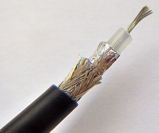
In electrical engineering, a transmission line is a specialized cable or other structure designed to conduct electromagnetic waves in a contained manner. The term applies when the conductors are long enough that the wave nature of the transmission must be taken into account. This applies especially to radio-frequency engineering because the short wavelengths mean that wave phenomena arise over very short distances. However, the theory of transmission lines was historically developed to explain phenomena on very long telegraph lines, especially submarine telegraph cables.

<span class="mw-page-title-main">Electrical impedance</span> Opposition of a circuit to a current when a voltage is applied

In electrical engineering, impedance is the opposition to alternating current presented by the combined effect of resistance and reactance in a circuit.

<span class="mw-page-title-main">Navier–Stokes equations</span> Equations describing the motion of viscous fluid substances

The Navier–Stokes equations are partial differential equations which describe the motion of viscous fluid substances. They were named after French engineer and physicist Claude-Louis Navier and the Irish physicist and mathematician George Gabriel Stokes. They were developed over several decades of progressively building the theories, from 1822 (Navier) to 1842–1850 (Stokes).

<span class="mw-page-title-main">Poynting vector</span> Measure of directional electromagnetic energy flux

In physics, the Poynting vector represents the directional energy flux or power flow of an electromagnetic field. The SI unit of the Poynting vector is the watt per square metre (W/m2); kg/s3 in base SI units. It is named after its discoverer John Henry Poynting who first derived it in 1884. Nikolay Umov is also credited with formulating the concept. Oliver Heaviside also discovered it independently in the more general form that recognises the freedom of adding the curl of an arbitrary vector field to the definition. The Poynting vector is used throughout electromagnetics in conjunction with Poynting's theorem, the continuity equation expressing conservation of electromagnetic energy, to calculate the power flow in electromagnetic fields.

In electrical circuits, reactance is the opposition presented to alternating current by inductance and capacitance. Along with resistance, it is one of two elements of impedance; however, while both elements involve transfer of electrical energy, no dissipation of electrical energy as heat occurs in reactance; instead, the reactance stores energy until a quarter-cycle later when the energy is returned to the circuit. Greater reactance gives smaller current for the same applied voltage.

<span class="mw-page-title-main">Moment of inertia</span> Scalar measure of the rotational inertia with respect to a fixed axis of rotation

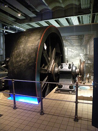
The moment of inertia, otherwise known as the mass moment of inertia, angular/rotational mass, second moment of mass, or most accurately, rotational inertia, of a rigid body is a quantity that determines the torque needed for a desired angular acceleration about a rotational axis, akin to how mass determines the force needed for a desired acceleration. It depends on the body's mass distribution and the axis chosen, with larger moments requiring more torque to change the body's rate of rotation by a given amount.

<span class="mw-page-title-main">Inductance</span> Property of electrical conductors

Inductance is the tendency of an electrical conductor to oppose a change in the electric current flowing through it. The electric current produces a magnetic field around the conductor. The magnetic field strength depends on the magnitude of the electric current, and follows any changes in the magnitude of the current. From Faraday's law of induction, any change in magnetic field through a circuit induces an electromotive force (EMF) (voltage) in the conductors, a process known as electromagnetic induction. This induced voltage created by the changing current has the effect of opposing the change in current. This is stated by Lenz's law, and the voltage is called back EMF.

<span class="mw-page-title-main">Dipole antenna</span> Antenna consisting of two rod shaped conductors

In radio and telecommunications a dipole antenna or doublet is one of the two simplest and most widely-used types of antenna; the other is the monopole. The dipole is any one of a class of antennas producing a radiation pattern approximating that of an elementary electric dipole with a radiating structure supporting a line current so energized that the current has only one node at each far end. A dipole antenna commonly consists of two identical conductive elements such as metal wires or rods. The driving current from the transmitter is applied, or for receiving antennas the output signal to the receiver is taken, between the two halves of the antenna. Each side of the feedline to the transmitter or receiver is connected to one of the conductors. This contrasts with a monopole antenna, which consists of a single rod or conductor with one side of the feedline connected to it, and the other side connected to some type of ground. A common example of a dipole is the "rabbit ears" television antenna found on broadcast television sets. All dipoles are electrically equivalent to two monopoles mounted end-to-end and fed with opposite phases, with the ground plane between them made "virtual" by the opposing monopole.

Acoustic impedance and specific acoustic impedance are measures of the opposition that a system presents to the acoustic flow resulting from an acoustic pressure applied to the system. The SI unit of acoustic impedance is the pascal-second per cubic metre, or in the MKS system the rayl per square metre (Rayl/m2), while that of specific acoustic impedance is the pascal-second per metre (Pa·s/m), or in the MKS system the rayl (Rayl). There is a close analogy with electrical impedance, which measures the opposition that a system presents to the electric current resulting from a voltage applied to the system.

<span class="mw-page-title-main">LC circuit</span> Electrical "resonator" circuit, consisting of inductive and capacitive elements with no resistance

An LC circuit, also called a resonant circuit, tank circuit, or tuned circuit, is an electric circuit consisting of an inductor, represented by the letter L, and a capacitor, represented by the letter C, connected together. The circuit can act as an electrical resonator, an electrical analogue of a tuning fork, storing energy oscillating at the circuit's resonant frequency.

A resistor–inductor circuit, or RL filter or RL network, is an electric circuit composed of resistors and inductors driven by a voltage or current source. A first-order RL circuit is composed of one resistor and one inductor, either in series driven by a voltage source or in parallel driven by a current source. It is one of the simplest analogue infinite impulse response electronic filters.

<span class="mw-page-title-main">Cartesian tensor</span>

In geometry and linear algebra, a Cartesian tensor uses an orthonormal basis to represent a tensor in a Euclidean space in the form of components. Converting a tensor's components from one such basis to another is done through an orthogonal transformation.

The electromagnetic wave equation is a second-order partial differential equation that describes the propagation of electromagnetic waves through a medium or in a vacuum. It is a three-dimensional form of the wave equation. The homogeneous form of the equation, written in terms of either the electric field E or the magnetic field B, takes the form:

<span class="mw-page-title-main">Electrical resonance</span> Canceling impedances at a particular frequency

Electrical resonance occurs in an electric circuit at a particular resonant frequency when the impedances or admittances of circuit elements cancel each other. In some circuits, this happens when the impedance between the input and output of the circuit is almost zero and the transfer function is close to one.

The derivatives of scalars, vectors, and second-order tensors with respect to second-order tensors are of considerable use in continuum mechanics. These derivatives are used in the theories of nonlinear elasticity and plasticity, particularly in the design of algorithms for numerical simulations.

In physics, slowly varying envelope approximation is the assumption that the envelope of a forward-travelling wave pulse varies slowly in time and space compared to a period or wavelength. This requires the spectrum of the signal to be narrow-banded—hence it is also referred to as the narrow-band approximation.

<span class="mw-page-title-main">Stokes' theorem</span> Theorem in vector calculus

Stokes' theorem, also known as the Kelvin–Stokes theorem after Lord Kelvin and George Stokes, the fundamental theorem for curls or simply the curl theorem, is a theorem in vector calculus on . Given a vector field, the theorem relates the integral of the curl of the vector field over some surface, to the line integral of the vector field around the boundary of the surface. The classical theorem of Stokes can be stated in one sentence: The line integral of a vector field over a loop is equal to the surface integral of its curl over the enclosed surface. It is illustrated in the figure, where the direction of positive circulation of the bounding contour ∂Σ, and the direction n of positive flux through the surface Σ, are related by a right-hand-rule. For the right hand the fingers circulate along ∂Σ and the thumb is directed along n.

References

  1. 1 2 3 Hayt, William H. (1989). Engineering Electromagnetics (5th ed.). McGraw-Hill. pp. 381–392. ISBN   0070274061 via Internet Archive (archive.org).
  2. 1 2 Johnson, Howard; Graham, Martin (2003). High Speed Signal Propagation (1st ed.). Prentice-Hall. ISBN   0-13-084408-X.
  3. Hunt, Bruce J. (2005). The Maxwellians. Ithaca, NY, USA: Cornell University Press. pp. 66–67. ISBN   0-80148234-8.
  4. Reeve, Whitman D. (1995). Subscriber Loop Signaling and Transmission Handbook. IEEE Press. p. 558. ISBN   0-7803-0440-3.
  5. Terman, Frederick Emmons (1943). Radio Engineers' Handbook (1st ed.). McGraw-Hill. p. 112.
  6. Chen, Walter Y. (2004). Home Networking Basics. Prentice Hall. p. 26. ISBN   0-13-016511-5.
  7. Kraus, John D. (1984). Electromagnetics (3rd ed.). McGraw-Hill. pp. 380–419. ISBN   0-07-035423-5.
  8. 1 2 Marshall, Stanley V.; Skitek, Gabriel G. (1987). Electromagnetic Concepts and Applications (2nd ed.). Prentice-Hall. ISBN   0-13-249004-8.
  9. 1 2 Sadiku, Matthew N.O. (1989). Elements of Electromagnetics (1st ed.). Saunders College Publishing. ISBN   0-03-013484-6.
  10. Harrington, Roger F. (1961). Time-Harmonic Electromagnetic Fields (1st ed.). McGraw-Hill. pp. 61–65. ISBN   0-07-026745-6.
  11. 1 2 Karakash, John J. (1950). Transmission lines and Filter Networks (1st ed.). Macmillan. pp. 5–14.
  12. Metzger, Georges; Vabre, Jean-Paul (1969). Transmission Lines with Pulse Excitation (1st ed.). Academic Press. pp. 1–10. LCCN   69-18342.
  13. Miano, Giovanni; Maffucci, Antonio (2001). Transmission Lines and Lumped Circuits. Academic Press. p. 130. ISBN   0-12-189710-9. The book uses the symbol μ instead of α.
  14. McCammon, Roy (June 2010). "SPICE Simulation of Transmission Lines by the Telegrapher's Method" (PDF). cmpnet.com. RF Design Line. Retrieved 2010-10-22; also = microwave-rf-design "Part 1 of 3". SPICE simulation of transmission lines by the telegrapher's method. Microwave & RF design via E.E. Times.{{cite book}}: Check |section-url= value (help)