Transmission-line matrix method

Last updated

The transmission-line matrix (TLM) method is a space and time discretising method for computation of electromagnetic fields. It is based on the analogy between the electromagnetic field and a mesh of transmission lines. The TLM method allows the computation of complex three-dimensional electromagnetic structures and has proven to be one of the most powerful time-domain methods along with the finite difference time domain (FDTD) method. The TLM was first explored by Raymond Beurle while working at English Electric Valve Company in Chelmsford. After he had been appointed professor of electrical engineering at the University of Nottingham in 1963 he jointly authored an article, "Numerical solution of 2-dimensional scattering problems using a transmission-line matrix", with Peter B. Johns in 1971. [1]

Contents

Basic principle

2D TLM example: an incident voltage pulse in two consecutive scattering events. SingleNode2DTLM.png
2D TLM example: an incident voltage pulse in two consecutive scattering events.

The TLM method is based on Huygens' model of wave propagation and scattering and the analogy between field propagation and transmission lines. Therefore, it considers the computational domain as a mesh of transmission lines, interconnected at nodes. In the figure on the right is considered a simple example of a 2D TLM mesh with a voltage pulse of amplitude 1 V incident on the central node. This pulse will be partially reflected and transmitted according to the transmission-line theory. If we assume that each line has a characteristic impedance , then the incident pulse sees effectively three transmission lines in parallel with a total impedance of . The reflection coefficient and the transmission coefficient are given by

The energy injected into the node by the incident pulse and the total energy of the scattered pulses are correspondingly

Therefore, the energy conservation law is fulfilled by the model.

The next scattering event excites the neighbouring nodes according to the principle described above. It can be seen that every node turns into a secondary source of spherical wave. These waves combine to form the overall waveform. This is in accordance with Huygens principle of light propagation.

In order to show the TLM schema we will use time and space discretisation. The time-step will be denoted with and the space discretisation intervals with , and . The absolute time and space will therefore be , , , , where is the time instant and are the cell coordinates. In case the value will be used, which is the lattice constant. In this case the following holds:

where is the free space speed of light.

The 2D TLM node

The scattering matrix of an 2D TLM node

A 2D series TLM node SeriesTlmNode.png
A 2D series TLM node

If we consider an electromagnetic field distribution in which the only non-zero components are , and (i.e. a TE-mode distribution), then Maxwell's equations in Cartesian coordinates reduce to

We can combine these equations to obtain

The figure on the right presents a structure referred to as a series node. It describes a block of space dimensions , and that consists of four ports. and are the distributed inductance and capacitance of the transmission lines. It is possible to show that a series node is equivalent to a TE-wave, more precisely the mesh current I, the x-direction voltages (ports 1 and 3) and the y-direction voltages (ports 2 and 4) may be related to the field components , and . If the voltages on the ports are considered, , and the polarity from the above figure holds, then the following is valid

where .

and dividing both sides by

Since and substituting gives

This reduces to Maxwell's equations when .

Similarly, using the conditions across the capacitors on ports 1 and 4, it can be shown that the corresponding two other Maxwell equations are the following:

Having these results, it is possible to compute the scattering matrix of a shunt node. The incident voltage pulse on port 1 at time-step k is denoted as . Replacing the four line segments from the above figure with their Thevenin equivalent it is possible to show that the following equation for the reflected voltage pulse holds:

If all incident waves as well as all reflected waves are collected in one vector, then this equation may be written down for all ports in matrix form:

where and are the incident and the reflected pulse amplitude vectors.

For a series node the scattering matrix S has the following form

Connection between TLM nodes

A 2D series TLM node 2DTLMmes.png
A 2D series TLM node

In order to describe the connection between adjacent nodes by a mesh of series nodes, look at the figure on the right. As the incident pulse in timestep k+1 on a node is the scattered pulse from an adjacent node in timestep k, the following connection equations are derived:

By modifying the scattering matrix inhomogeneous and lossy materials can be modelled. By adjusting the connection equations it is possible to simulate different boundaries.

The shunt TLM node

Apart from the series node, described above there is also the shunt TLM node, which represents a TM-mode field distribution. The only non-zero components of such wave are , , and . With similar considerations as for the series node the scattering matrix of the shunt node can be derived.

3D TLM models

A 3D symmetric condensed node SymmetricCondensedNode.png
A 3D symmetric condensed node

Most problems in electromagnetics require a three-dimensional grid. As we now have structures that describe TE and TM-field distributions, intuitively it seems possible to define a combination of shunt and series nodes providing a full description of the electromagnetic field. Such attempts have been made, but because of the complexity of the resulting structures they proved to be not very useful. Using the analogy that was presented above leads to calculation of the different field components at physically separated points. This causes difficulties in providing simple and efficient boundary definitions. A solution to these problems was provided by Johns in 1987, when he proposed the structure known as the symmetrical condensed node (SCN), presented in the figure on the right. It consists of 12 ports because two field polarisations are to be assigned to each of the 6 sides of a mesh cell.

The topology of the SCN cannot be analysed using Thevenin equivalent circuits. More general energy and charge conservation principles are to be used.

The electric and the magnetic fields on the sides of the SCN node number (l,m,n) at time instant k may be summarised in 12-dimensional vectors

They can be linked with the incident and scattered amplitude vectors via

where is the field impedance, is the vector of the amplitudes of the incident waves to the node, and is the vector of the scattered amplitudes. The relation between the incident and scattered waves is given by the matrix equation

The scattering matrix S can be calculated. For the symmetrical condensed node with ports defined as in the figure the following result is obtained

where the following matrix was used

The connection between different SCNs is done in the same manner as for the 2D nodes.

Open-sourced code implementation of 3D-TLM

The George Green Institute for Electromagnetics Research (GGIEMR) has open-sourced an efficient implementation of 3D-TLM, capable of parallel computation by means of MPI named GGITLM and available online. [2]

Related Research Articles

<span class="mw-page-title-main">Wave equation</span> Differential equation important in physics

The wave equation is a second-order linear partial differential equation for the description of waves or standing wave fields such as mechanical waves or electromagnetic waves. It arises in fields like acoustics, electromagnetism, and fluid dynamics.

<span class="mw-page-title-main">Moment of inertia</span> Scalar measure of the rotational inertia with respect to a fixed axis of rotation

The moment of inertia, otherwise known as the mass moment of inertia, angular mass, second moment of mass, or most accurately, rotational inertia, of a rigid body is a quantity that determines the torque needed for a desired angular acceleration about a rotational axis, akin to how mass determines the force needed for a desired acceleration. It depends on the body's mass distribution and the axis chosen, with larger moments requiring more torque to change the body's rate of rotation by a given amount.

<span class="mw-page-title-main">Heat equation</span> Partial differential equation describing the evolution of temperature in a region

In mathematics and physics, the heat equation is a certain partial differential equation. Solutions of the heat equation are sometimes known as caloric functions. The theory of the heat equation was first developed by Joseph Fourier in 1822 for the purpose of modeling how a quantity such as heat diffuses through a given region.

In mathematics, the Laplace operator or Laplacian is a differential operator given by the divergence of the gradient of a scalar function on Euclidean space. It is usually denoted by the symbols , (where is the nabla operator), or . In a Cartesian coordinate system, the Laplacian is given by the sum of second partial derivatives of the function with respect to each independent variable. In other coordinate systems, such as cylindrical and spherical coordinates, the Laplacian also has a useful form. Informally, the Laplacian Δf (p) of a function f at a point p measures by how much the average value of f over small spheres or balls centered at p deviates from f (p).

<span class="mw-page-title-main">Spherical harmonics</span> Special mathematical functions defined on the surface of a sphere

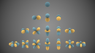
In mathematics and physical science, spherical harmonics are special functions defined on the surface of a sphere. They are often employed in solving partial differential equations in many scientific fields. A list of the spherical harmonics is available in Table of spherical harmonics.

In special relativity, four-momentum (also called momentum–energy or momenergy) is the generalization of the classical three-dimensional momentum to four-dimensional spacetime. Momentum is a vector in three dimensions; similarly four-momentum is a four-vector in spacetime. The contravariant four-momentum of a particle with relativistic energy E and three-momentum p = (px, py, pz) = γmv, where v is the particle's three-velocity and γ the Lorentz factor, is

In vector calculus, Green's theorem relates a line integral around a simple closed curve C to a double integral over the plane region D bounded by C. It is the two-dimensional special case of Stokes' theorem.

<span class="mw-page-title-main">Product rule</span> Formula for the derivative of a product

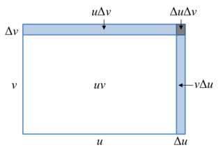
In calculus, the product rule is a formula used to find the derivatives of products of two or more functions. For two functions, it may be stated in Lagrange's notation as

In mathematics, the Hodge star operator or Hodge star is a linear map defined on the exterior algebra of a finite-dimensional oriented vector space endowed with a nondegenerate symmetric bilinear form. Applying the operator to an element of the algebra produces the Hodge dual of the element. This map was introduced by W. V. D. Hodge.

In analytical mechanics, generalized coordinates are a set of parameters used to represent the state of a system in a configuration space. These parameters must uniquely define the configuration of the system relative to a reference state. The generalized velocities are the time derivatives of the generalized coordinates of the system. The adjective "generalized" distinguishes these parameters from the traditional use of the term "coordinate" to refer to Cartesian coordinates.

In physics, the Hamilton–Jacobi equation, named after William Rowan Hamilton and Carl Gustav Jacob Jacobi, is an alternative formulation of classical mechanics, equivalent to other formulations such as Newton's laws of motion, Lagrangian mechanics and Hamiltonian mechanics.

In quantum physics, the spin–orbit interaction is a relativistic interaction of a particle's spin with its motion inside a potential. A key example of this phenomenon is the spin–orbit interaction leading to shifts in an electron's atomic energy levels, due to electromagnetic interaction between the electron's magnetic dipole, its orbital motion, and the electrostatic field of the positively charged nucleus. This phenomenon is detectable as a splitting of spectral lines, which can be thought of as a Zeeman effect product of two relativistic effects: the apparent magnetic field seen from the electron perspective and the magnetic moment of the electron associated with its intrinsic spin. A similar effect, due to the relationship between angular momentum and the strong nuclear force, occurs for protons and neutrons moving inside the nucleus, leading to a shift in their energy levels in the nucleus shell model. In the field of spintronics, spin–orbit effects for electrons in semiconductors and other materials are explored for technological applications. The spin–orbit interaction is at the origin of magnetocrystalline anisotropy and the spin Hall effect.

<span class="mw-page-title-main">Electromagnetic tensor</span> Mathematical object that describes the electromagnetic field in spacetime

In electromagnetism, the electromagnetic tensor or electromagnetic field tensor is a mathematical object that describes the electromagnetic field in spacetime. The field tensor was first used after the four-dimensional tensor formulation of special relativity was introduced by Hermann Minkowski. The tensor allows related physical laws to be written very concisely, and allows for the quantization of the electromagnetic field by Lagrangian formulation described below.

The electromagnetic wave equation is a second-order partial differential equation that describes the propagation of electromagnetic waves through a medium or in a vacuum. It is a three-dimensional form of the wave equation. The homogeneous form of the equation, written in terms of either the electric field E or the magnetic field B, takes the form:

<span class="mw-page-title-main">Covariant formulation of classical electromagnetism</span> Ways of writing certain laws of physics

The covariant formulation of classical electromagnetism refers to ways of writing the laws of classical electromagnetism in a form that is manifestly invariant under Lorentz transformations, in the formalism of special relativity using rectilinear inertial coordinate systems. These expressions both make it simple to prove that the laws of classical electromagnetism take the same form in any inertial coordinate system, and also provide a way to translate the fields and forces from one frame to another. However, this is not as general as Maxwell's equations in curved spacetime or non-rectilinear coordinate systems.

In mathematics, vector spherical harmonics (VSH) are an extension of the scalar spherical harmonics for use with vector fields. The components of the VSH are complex-valued functions expressed in the spherical coordinate basis vectors.

<span class="mw-page-title-main">Lagrangian mechanics</span> Formulation of classical mechanics

In physics, Lagrangian mechanics is a formulation of classical mechanics founded on the stationary-action principle. It was introduced by the Italian-French mathematician and astronomer Joseph-Louis Lagrange in his presentation to the Turin Academy of Science in 1760 culminating in his 1788 grand opus, Mécanique analytique.

The quantization of the electromagnetic field means that an electromagnetic field consists of discrete energy parcels called photons. Photons are massless particles of definite energy, definite momentum, and definite spin.

<span class="mw-page-title-main">Relativistic angular momentum</span> Angular momentum in special and general relativity

In physics, relativistic angular momentum refers to the mathematical formalisms and physical concepts that define angular momentum in special relativity (SR) and general relativity (GR). The relativistic quantity is subtly different from the three-dimensional quantity in classical mechanics.

Lagrangian field theory is a formalism in classical field theory. It is the field-theoretic analogue of Lagrangian mechanics. Lagrangian mechanics is used to analyze the motion of a system of discrete particles each with a finite number of degrees of freedom. Lagrangian field theory applies to continua and fields, which have an infinite number of degrees of freedom.

References

  1. de Cogan, Donard (12 December 2018). Transmission Line Matrix (TLM) Techniques for Diffusion Applications. Routledge. ISBN   978-1-351-40712-0.
  2. "George Green Institute for Electromagnetics Research - TLM time domain simulation code". University of Nottingham - George Green Institute for Electromagnetics Research. University of Nottingham. Retrieved 23 March 2017.