Tree decomposition

Last updated
A graph with eight vertices, and a tree decomposition of it onto a tree with six nodes. Each graph edge connects two vertices that are listed together at some tree node, and each graph vertex is listed at the nodes of a contiguous subtree of the tree. Each tree node lists at most three vertices, so the width of this decomposition is two. Tree decomposition.svg
A graph with eight vertices, and a tree decomposition of it onto a tree with six nodes. Each graph edge connects two vertices that are listed together at some tree node, and each graph vertex is listed at the nodes of a contiguous subtree of the tree. Each tree node lists at most three vertices, so the width of this decomposition is two.

In graph theory, a tree decomposition is a mapping of a graph into a tree that can be used to define the treewidth of the graph and speed up solving certain computational problems on the graph.

Contents

Tree decompositions are also called junction trees, clique trees, or join trees. They play an important role in problems like probabilistic inference, constraint satisfaction, query optimization, [1] and matrix decomposition.

The concept of tree decomposition was originally introduced by RudolfHalin  ( 1976 ). Later it was rediscovered by NeilRobertson and Paul Seymour  ( 1984 ) and has since been studied by many other authors. [2]

Definition

Intuitively, a tree decomposition represents the vertices of a given graph G as subtrees of a tree, in such a way that vertices in G are adjacent only when the corresponding subtrees intersect. Thus, G forms a subgraph of the intersection graph of the subtrees. The full intersection graph is a chordal graph.

Each subtree associates a graph vertex with a set of tree nodes. To define this formally, we represent each tree node as the set of vertices associated with it. Thus, given a graph G = (V, E), a tree decomposition is a pair (X, T), where X = {X1, …, Xn} is a family of subsets (sometimes called bags) of V, and T is a tree whose nodes are the subsets Xi, satisfying the following properties: [3]

  1. The union of all sets Xi equals V. That is, each graph vertex is associated with at least one tree node.
  2. For every edge (v, w) in the graph, there is a subset Xi that contains both v and w. That is, vertices are adjacent in the graph only when the corresponding subtrees have a node in common.
  3. If Xi and Xj both contain a vertex v, then all nodes Xk of the tree in the (unique) path between Xi and Xj contain v as well. That is, the nodes associated with vertex v form a connected subset of T. This is also known as coherence, or the running intersection property. It can be stated equivalently that if Xi, Xj and Xk are nodes, and Xk is on the path from Xi to Xj, then .

The tree decomposition of a graph is far from unique; for example, a trivial tree decomposition contains all vertices of the graph in its single root node.

A tree decomposition in which the underlying tree is a path graph is called a path decomposition, and the width parameter derived from these special types of tree decompositions is known as pathwidth.

A tree decomposition (X, T = (I, F)) of treewidth k is smooth, if for all , and for all . [4]

Treewidth

Two different tree-decompositions of the same graph Treedecompsnocolour.JPG
Two different tree-decompositions of the same graph

The width of a tree decomposition is the size of its largest set Xi minus one. The treewidth tw(G) of a graph G is the minimum width among all possible tree decompositions of G. In this definition, the size of the largest set is diminished by one in order to make the treewidth of a tree equal to one. Treewidth may also be defined from other structures than tree decompositions, including chordal graphs, brambles, and havens.

It is NP-complete to determine whether a given graph G has treewidth at most a given variable k. [5] However, when k is any fixed constant, the graphs with treewidth k can be recognized, and a width k tree decomposition constructed for them, in linear time. [4] The time dependence of this algorithm on k is an exponential function of k3.

Dynamic programming

At the beginning of the 1970s, it was observed that a large class of combinatorial optimization problems defined on graphs could be efficiently solved by non-serial dynamic programming as long as the graph had a bounded dimension, [6] a parameter related to treewidth. Later, several authors independently observed, at the end of the 1980s, [7] that many algorithmic problems that are NP-complete for arbitrary graphs may be solved efficiently by dynamic programming for graphs of bounded treewidth, using the tree-decompositions of these graphs.

As an example, consider the problem of finding the maximum independent set in a graph of treewidth k. To solve this problem, first choose one of the nodes of the tree decomposition to be the root, arbitrarily. For a node Xi of the tree decomposition, let Di be the union of the sets Xj descending from Xi. For an independent set let A(S,i) denote the size of the largest independent subset I of Di such that Similarly, for an adjacent pair of nodes Xi and Xj, with Xi farther from the root of the tree than Xj, and an independent set let B(S,i,j) denote the size of the largest independent subset I of Di such that We may calculate these A and B values by a bottom-up traversal of the tree:

where the sum in the calculation of is over the children of node Xi.

At each node or edge, there are at most 2k sets S for which we need to calculate these values, so if k is a constant then the whole calculation takes constant time per edge or node. The size of the maximum independent set is the largest value stored at the root node, and the maximum independent set itself can be found (as is standard in dynamic programming algorithms) by backtracking through these stored values starting from this largest value. Thus, in graphs of bounded treewidth, the maximum independent set problem may be solved in linear time. Similar algorithms apply to many other graph problems.

This dynamic programming approach is used in machine learning via the junction tree algorithm for belief propagation in graphs of bounded treewidth. It also plays a key role in algorithms for computing the treewidth and constructing tree decompositions: typically, such algorithms have a first step that approximates the treewidth, constructing a tree decomposition with this approximate width, and then a second step that performs dynamic programming in the approximate tree decomposition to compute the exact value of the treewidth. [4]

See also

Notes

  1. Gottlob et al. (2012).
  2. Diestel (2005) pp.354–355
  3. Diestel (2005) section 12.3
  4. 1 2 3 Bodlaender (1996).
  5. Arnborg, Corneil & Proskurowski (1987).
  6. Bertelé & Brioschi (1972).
  7. Arnborg & Proskurowski (1989); Bern, Lawler & Wong (1987); Bodlaender (1988).

Related Research Articles

This is a glossary of graph theory. Graph theory is the study of graphs, systems of nodes or vertices connected in pairs by lines or edges.

<span class="mw-page-title-main">Chordal graph</span> Graph where all long cycles have a chord

In the mathematical area of graph theory, a chordal graph is one in which all cycles of four or more vertices have a chord, which is an edge that is not part of the cycle but connects two vertices of the cycle. Equivalently, every induced cycle in the graph should have exactly three vertices. The chordal graphs may also be characterized as the graphs that have perfect elimination orderings, as the graphs in which each minimal separator is a clique, and as the intersection graphs of subtrees of a tree. They are sometimes also called rigid circuit graphs or triangulated graphs: a chordal completion of a graph is typically called a triangulation of that graph.

In mathematics, in the areas of order theory and combinatorics, Dilworth's theorem characterizes the width of any finite partially ordered set in terms of a partition of the order into a minimum number of chains. It is named for the mathematician Robert P. Dilworth.

<span class="mw-page-title-main">Monochromatic triangle</span>

In graph theory and theoretical computer science, the monochromatic triangle problem is an algorithmic problem on graphs, in which the goal is to partition the edges of a given graph into two triangle-free subgraphs. It is NP-complete but fixed-parameter tractable on graphs of bounded treewidth.

In constraint satisfaction, local consistency conditions are properties of constraint satisfaction problems related to the consistency of subsets of variables or constraints. They can be used to reduce the search space and make the problem easier to solve. Various kinds of local consistency conditions are leveraged, including node consistency, arc consistency, and path consistency.

In graph theory, the treewidth of an undirected graph is an integer number which specifies, informally, how far the graph is from being a tree. The smallest treewidth is 1; the graphs with treewidth 1 are exactly the trees and the forests. The graphs with treewidth at most 2 are the series–parallel graphs. The maximal graphs with treewidth exactly k are called k-trees, and the graphs with treewidth at most k are called partial k-trees. Many other well-studied graph families also have bounded treewidth.

In constraint satisfaction, a decomposition method translates a constraint satisfaction problem into another constraint satisfaction problem that is binary and acyclic. Decomposition methods work by grouping variables into sets, and solving a subproblem for each set. These translations are done because solving binary acyclic problems is a tractable problem.

In graph theory, a path decomposition of a graph G is, informally, a representation of G as a "thickened" path graph, and the pathwidth of G is a number that measures how much the path was thickened to form G. More formally, a path-decomposition is a sequence of subsets of vertices of G such that the endpoints of each edge appear in one of the subsets and such that each vertex appears in a contiguous subsequence of the subsets, and the pathwidth is one less than the size of the largest set in such a decomposition. Pathwidth is also known as interval thickness, vertex separation number, or node searching number.

<span class="mw-page-title-main">Series–parallel graph</span> Recursively-formed graph with two terminal vertices

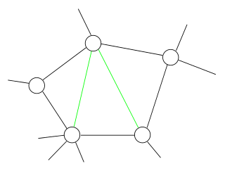
In graph theory, series–parallel graphs are graphs with two distinguished vertices called terminals, formed recursively by two simple composition operations. They can be used to model series and parallel electric circuits.

<span class="mw-page-title-main">Branch-decomposition</span> Hierarchical clustering of graph edges

In graph theory, a branch-decomposition of an undirected graph G is a hierarchical clustering of the edges of G, represented by an unrooted binary tree T with the edges of G as its leaves. Removing any edge from T partitions the edges of G into two subgraphs, and the width of the decomposition is the maximum number of shared vertices of any pair of subgraphs formed in this way. The branchwidth of G is the minimum width of any branch-decomposition of G.

In graph theory, the planar separator theorem is a form of isoperimetric inequality for planar graphs, that states that any planar graph can be split into smaller pieces by removing a small number of vertices. Specifically, the removal of vertices from an n-vertex graph can partition the graph into disjoint subgraphs each of which has at most vertices.

In graph theory, the tree-depth of a connected undirected graph is a numerical invariant of , the minimum height of a Trémaux tree for a supergraph of . This invariant and its close relatives have gone under many different names in the literature, including vertex ranking number, ordered chromatic number, and minimum elimination tree height; it is also closely related to the cycle rank of directed graphs and the star height of regular languages. Intuitively, where the treewidth of a graph measures how far it is from being a tree, this parameter measures how far a graph is from being a star.

<span class="mw-page-title-main">Unrooted binary tree</span>

In mathematics and computer science, an unrooted binary tree is an unrooted tree in which each vertex has either one or three neighbors.

In graph theory, the modular decomposition is a decomposition of a graph into subsets of vertices called modules. A module is a generalization of a connected component of a graph. Unlike connected components, however, one module can be a proper subset of another. Modules therefore lead to a recursive (hierarchical) decomposition of the graph, instead of just a partition.

In graph theory, a partial k-tree is a type of graph, defined either as a subgraph of a k-tree or as a graph with treewidth at most k. Many NP-hard combinatorial problems on graphs are solvable in polynomial time when restricted to the partial k-trees, for bounded values of k.

In the study of graph algorithms, Courcelle's theorem is the statement that every graph property definable in the monadic second-order logic of graphs can be decided in linear time on graphs of bounded treewidth. The result was first proved by Bruno Courcelle in 1990 and independently rediscovered by Borie, Parker & Tovey (1992). It is considered the archetype of algorithmic meta-theorems.

<span class="mw-page-title-main">Bramble (graph theory)</span> Method of graph decomposition

In graph theory, a bramble for an undirected graph G is a family of connected subgraphs of G that all touch each other: for every pair of disjoint subgraphs, there must exist an edge in G that has one endpoint in each subgraph. The order of a bramble is the smallest size of a hitting set, a set of vertices of G that has a nonempty intersection with each of the subgraphs. Brambles may be used to characterize the treewidth of G.

In the mathematical field of graph theory, an agreement forest for two given trees is any forest which can, informally speaking, be obtained from both trees by removing a common number of edges.

<span class="mw-page-title-main">Cutwidth</span> Property in graph theory

In graph theory, the cutwidth of an undirected graph is the smallest integer with the following property: there is an ordering of the vertices of the graph, such that every cut obtained by partitioning the vertices into earlier and later subsets of the ordering is crossed by at most edges. That is, if the vertices are numbered , then for every , the number of edges with and is at most .

In graph theory, the carving width of a graph is a number, defined from the graph, that describes the number of edges separating the clusters in a hierarchical clustering of the graph vertices.

References