Bra–ket notation, also called Dirac notation, is a notation for linear algebra and linear operators on complex vector spaces together with their dual space both in the finite-dimensional and infinite-dimensional case. It is specifically designed to ease the types of calculations that frequently come up in quantum mechanics. Its use in quantum mechanics is quite widespread.

In theoretical physics, a Feynman diagram is a pictorial representation of the mathematical expressions describing the behavior and interaction of subatomic particles. The scheme is named after American physicist Richard Feynman, who introduced the diagrams in 1948. The interaction of subatomic particles can be complex and difficult to understand; Feynman diagrams give a simple visualization of what would otherwise be an arcane and abstract formula. According to David Kaiser, "Since the middle of the 20th century, theoretical physicists have increasingly turned to this tool to help them undertake critical calculations. Feynman diagrams have revolutionized nearly every aspect of theoretical physics." While the diagrams are applied primarily to quantum field theory, they can also be used in other areas of physics, such as solid-state theory. Frank Wilczek wrote that the calculations that won him the 2004 Nobel Prize in Physics "would have been literally unthinkable without Feynman diagrams, as would [Wilczek's] calculations that established a route to production and observation of the Higgs particle."

The proof of Gödel's completeness theorem given by Kurt Gödel in his doctoral dissertation of 1929 is not easy to read today; it uses concepts and formalisms that are no longer used and terminology that is often obscure. The version given below attempts to represent all the steps in the proof and all the important ideas faithfully, while restating the proof in the modern language of mathematical logic. This outline should not be considered a rigorous proof of the theorem.

In statistics, a normal distribution or Gaussian distribution is a type of continuous probability distribution for a real-valued random variable. The general form of its probability density function is
Shor's algorithm is a quantum algorithm for finding the prime factors of an integer. It was developed in 1994 by the American mathematician Peter Shor. It is one of the few known quantum algorithms with compelling potential applications and strong evidence of superpolynomial speedup compared to best known classical algorithms. On the other hand, factoring numbers of practical significance requires far more qubits than available in the near future. Another concern is that noise in quantum circuits may undermine results, requiring additional qubits for quantum error correction.
A Bayesian network is a probabilistic graphical model that represents a set of variables and their conditional dependencies via a directed acyclic graph (DAG). While it is one of several forms of causal notation, causal networks are special cases of Bayesian networks. Bayesian networks are ideal for taking an event that occurred and predicting the likelihood that any one of several possible known causes was the contributing factor. For example, a Bayesian network could represent the probabilistic relationships between diseases and symptoms. Given symptoms, the network can be used to compute the probabilities of the presence of various diseases.
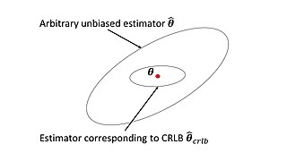
In estimation theory and statistics, the Cramér–Rao bound (CRB) relates to estimation of a deterministic parameter. The result is named in honor of Harald Cramér and C. R. Rao, but has also been derived independently by Maurice Fréchet, Georges Darmois, and by Alexander Aitken and Harold Silverstone. It is also known as Fréchet-Cramér–Rao or Fréchet-Darmois-Cramér-Rao lower bound. It states that the precision of any unbiased estimator is at most the Fisher information; or (equivalently) the reciprocal of the Fisher information is a lower bound on its variance.
The Gram–Charlier A series, and the Edgeworth series are series that approximate a probability distribution in terms of its cumulants. The series are the same; but, the arrangement of terms differ. The key idea of these expansions is to write the characteristic function of the distribution whose probability density function f is to be approximated in terms of the characteristic function of a distribution with known and suitable properties, and to recover f through the inverse Fourier transform.
In statistics, a mixture model is a probabilistic model for representing the presence of subpopulations within an overall population, without requiring that an observed data set should identify the sub-population to which an individual observation belongs. Formally a mixture model corresponds to the mixture distribution that represents the probability distribution of observations in the overall population. However, while problems associated with "mixture distributions" relate to deriving the properties of the overall population from those of the sub-populations, "mixture models" are used to make statistical inferences about the properties of the sub-populations given only observations on the pooled population, without sub-population identity information. Mixture models are used for clustering, under the name model-based clustering, and also for density estimation.
In mathematics, particularly in functional analysis, a projection-valued measure is a function defined on certain subsets of a fixed set and whose values are self-adjoint projections on a fixed Hilbert space. A projection-valued measure (PVM) is formally similar to a real-valued measure, except that its values are self-adjoint projections rather than real numbers. As in the case of ordinary measures, it is possible to integrate complex-valued functions with respect to a PVM; the result of such an integration is a linear operator on the given Hilbert space.

In probability and statistics, the Dirichlet distribution (after Peter Gustav Lejeune Dirichlet), often denoted , is a family of continuous multivariate probability distributions parameterized by a vector of positive reals. It is a multivariate generalization of the beta distribution, hence its alternative name of multivariate beta distribution (MBD). Dirichlet distributions are commonly used as prior distributions in Bayesian statistics, and in fact, the Dirichlet distribution is the conjugate prior of the categorical distribution and multinomial distribution.
In complexity theory, the Karp–Lipton theorem states that if the Boolean satisfiability problem (SAT) can be solved by Boolean circuits with a polynomial number of logic gates, then
The following are important identities involving derivatives and integrals in vector calculus.

The folded normal distribution is a probability distribution related to the normal distribution. Given a normally distributed random variable X with mean μ and variance σ2, the random variable Y = |X| has a folded normal distribution. Such a case may be encountered if only the magnitude of some variable is recorded, but not its sign. The distribution is called "folded" because probability mass to the left of x = 0 is folded over by taking the absolute value. In the physics of heat conduction, the folded normal distribution is a fundamental solution of the heat equation on the half space; it corresponds to having a perfect insulator on a hyperplane through the origin.
In statistics, the inverse Wishart distribution, also called the inverted Wishart distribution, is a probability distribution defined on real-valued positive-definite matrices. In Bayesian statistics it is used as the conjugate prior for the covariance matrix of a multivariate normal distribution.
In probability theory and statistics, the Dirichlet-multinomial distribution is a family of discrete multivariate probability distributions on a finite support of non-negative integers. It is also called the Dirichlet compound multinomial distribution (DCM) or multivariate Pólya distribution. It is a compound probability distribution, where a probability vector p is drawn from a Dirichlet distribution with parameter vector , and an observation drawn from a multinomial distribution with probability vector p and number of trials n. The Dirichlet parameter vector captures the prior belief about the situation and can be seen as a pseudocount: observations of each outcome that occur before the actual data is collected. The compounding corresponds to a Pólya urn scheme. It is frequently encountered in Bayesian statistics, machine learning, empirical Bayes methods and classical statistics as an overdispersed multinomial distribution.

In probability and statistics, the truncated normal distribution is the probability distribution derived from that of a normally distributed random variable by bounding the random variable from either below or above. The truncated normal distribution has wide applications in statistics and econometrics.
In mathematical analysis, and especially in real, harmonic analysis and functional analysis, an Orlicz space is a type of function space which generalizes the Lp spaces. Like the Lp spaces, they are Banach spaces. The spaces are named for Władysław Orlicz, who was the first to define them in 1932.

In probability theory and statistics, the generalized chi-squared distribution is the distribution of a quadratic form of a multinormal variable, or a linear combination of different normal variables and squares of normal variables. Equivalently, it is also a linear sum of independent noncentral chi-square variables and a normal variable. There are several other such generalizations for which the same term is sometimes used; some of them are special cases of the family discussed here, for example the gamma distribution.
Lagrangian field theory is a formalism in classical field theory. It is the field-theoretic analogue of Lagrangian mechanics. Lagrangian mechanics is used to analyze the motion of a system of discrete particles each with a finite number of degrees of freedom. Lagrangian field theory applies to continua and fields, which have an infinite number of degrees of freedom.


