
Probability theory or probability calculus is the branch of mathematics concerned with probability. Although there are several different probability interpretations, probability theory treats the concept in a rigorous mathematical manner by expressing it through a set of axioms. Typically these axioms formalise probability in terms of a probability space, which assigns a measure taking values between 0 and 1, termed the probability measure, to a set of outcomes called the sample space. Any specified subset of the sample space is called an event.
In probability theory and statistics, a probability distribution is the mathematical function that gives the probabilities of occurrence of different possible outcomes for an experiment. It is a mathematical description of a random phenomenon in terms of its sample space and the probabilities of events.
A random variable is a mathematical formalization of a quantity or object which depends on random events. The term 'random variable' in its mathematical definition refers to neither randomness nor variability but instead is a mathematical function in which
In probability theory, a probability space or a probability triple is a mathematical construct that provides a formal model of a random process or "experiment". For example, one can define a probability space which models the throwing of a die.
In probability theory, there exist several different notions of convergence of sequences of random variables, including convergence in probability, convergence in distribution, and almost sure convergence. The different notions of convergence capture different properties about the sequence, with some notions of convergence being stronger than others. For example, convergence in distribution tells us about the limit distribution of a sequence of random variables. This is a weaker notion than convergence in probability, which tells us about the value a random variable will take, rather than just the distribution.
In probability and statistics, a Bernoulli process is a finite or infinite sequence of binary random variables, so it is a discrete-time stochastic process that takes only two values, canonically 0 and 1. The component Bernoulli variablesXi are identically distributed and independent. Prosaically, a Bernoulli process is a repeated coin flipping, possibly with an unfair coin. Every variable Xi in the sequence is associated with a Bernoulli trial or experiment. They all have the same Bernoulli distribution. Much of what can be said about the Bernoulli process can also be generalized to more than two outcomes ; this generalization is known as the Bernoulli scheme.
In probability theory, the law of large numbers (LLN) is a mathematical theorem that states that the average of the results obtained from a large number of independent random samples converges to the true value, if it exists. More formally, the LLN states that given a sample of independent and identically distributed values, the sample mean converges to the true mean.
In probability theory, Kolmogorov's zero–one law, named in honor of Andrey Nikolaevich Kolmogorov, specifies that a certain type of event, namely a tail event of independent σ-algebras, will either almost surely happen or almost surely not happen; that is, the probability of such an event occurring is zero or one.
In information theory, the asymptotic equipartition property (AEP) is a general property of the output samples of a stochastic source. It is fundamental to the concept of typical set used in theories of data compression.
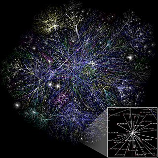
In mathematics, random graph is the general term to refer to probability distributions over graphs. Random graphs may be described simply by a probability distribution, or by a random process which generates them. The theory of random graphs lies at the intersection between graph theory and probability theory. From a mathematical perspective, random graphs are used to answer questions about the properties of typical graphs. Its practical applications are found in all areas in which complex networks need to be modeled – many random graph models are thus known, mirroring the diverse types of complex networks encountered in different areas. In a mathematical context, random graph refers almost exclusively to the Erdős–Rényi random graph model. In other contexts, any graph model may be referred to as a random graph.
In probability theory, the conditional expectation, conditional expected value, or conditional mean of a random variable is its expected value evaluated with respect to the conditional probability distribution. If the random variable can take on only a finite number of values, the "conditions" are that the variable can only take on a subset of those values. More formally, in the case when the random variable is defined over a discrete probability space, the "conditions" are a partition of this probability space.
In probability theory, random element is a generalization of the concept of random variable to more complicated spaces than the simple real line. The concept was introduced by Maurice Fréchet who commented that the “development of probability theory and expansion of area of its applications have led to necessity to pass from schemes where (random) outcomes of experiments can be described by number or a finite set of numbers, to schemes where outcomes of experiments represent, for example, vectors, functions, processes, fields, series, transformations, and also sets or collections of sets.”
In mathematics, a random compact set is essentially a compact set-valued random variable. Random compact sets are useful in the study of attractors for random dynamical systems.
The Hewitt–Savage zero–one law is a theorem in probability theory, similar to Kolmogorov's zero–one law and the Borel–Cantelli lemma, that specifies that a certain type of event will either almost surely happen or almost surely not happen. It is sometimes known as the Savage-Hewitt law for symmetric events. It is named after Edwin Hewitt and Leonard Jimmie Savage.

In probability theory and statistics, a sequence of independent Bernoulli trials with probability 1/2 of success on each trial is metaphorically called a fair coin. One for which the probability is not 1/2 is called a biased or unfair coin. In theoretical studies, the assumption that a coin is fair is often made by referring to an ideal coin.
In mathematics, uniform integrability is an important concept in real analysis, functional analysis and measure theory, and plays a vital role in the theory of martingales.
In probability theory, a standard probability space, also called Lebesgue–Rokhlin probability space or just Lebesgue space is a probability space satisfying certain assumptions introduced by Vladimir Rokhlin in 1940. Informally, it is a probability space consisting of an interval and/or a finite or countable number of atoms.
In mathematics – specifically, in the theory of stochastic processes – Doob's martingale convergence theorems are a collection of results on the limits of supermartingales, named after the American mathematician Joseph L. Doob. Informally, the martingale convergence theorem typically refers to the result that any supermartingale satisfying a certain boundedness condition must converge. One may think of supermartingales as the random variable analogues of non-increasing sequences; from this perspective, the martingale convergence theorem is a random variable analogue of the monotone convergence theorem, which states that any bounded monotone sequence converges. There are symmetric results for submartingales, which are analogous to non-decreasing sequences.
In the mathematical theory of probability, the Ionescu-Tulcea theorem, sometimes called the Ionesco Tulcea extension theorem, deals with the existence of probability measures for probabilistic events consisting of a countably infinite number of individual probabilistic events. In particular, the individual events may be independent or dependent with respect to each other. Thus, the statement goes beyond the mere existence of countable product measures. The theorem was proved by Cassius Ionescu-Tulcea in 1949.
In probability theory, the van den Berg–Kesten (BK) inequality or van den Berg–Kesten–Reimer (BKR) inequality states that the probability for two random events to both happen, and at the same time one can find "disjoint certificates" to show that they both happen, is at most the product of their individual probabilities. The special case for two monotone events was first proved by van den Berg and Kesten in 1985, who also conjectured that the inequality holds in general, not requiring monotonicity. Reimer later proved this conjecture. The inequality is applied to probability spaces with a product structure, such as in percolation problems.


