
In probability theory and statistics, the binomial distribution with parameters n and p is the discrete probability distribution of the number of successes in a sequence of n independent experiments, each asking a yes–no question, and each with its own Boolean-valued outcome: success or failure. A single success/failure experiment is also called a Bernoulli trial or Bernoulli experiment, and a sequence of outcomes is called a Bernoulli process; for a single trial, i.e., n = 1, the binomial distribution is a Bernoulli distribution. The binomial distribution is the basis for the popular binomial test of statistical significance.

In mathematics, the binomial coefficients are the positive integers that occur as coefficients in the binomial theorem. Commonly, a binomial coefficient is indexed by a pair of integers n ≥ k ≥ 0 and is written It is the coefficient of the xk term in the polynomial expansion of the binomial power (1 + x)n; this coefficient can be computed by the multiplicative formula

In probability theory and statistics, a normal distribution or Gaussian distribution is a type of continuous probability distribution for a real-valued random variable. The general form of its probability density function is
In probability theory, the central limit theorem (CLT) states that, under appropriate conditions, the distribution of a normalized version of the sample mean converges to a standard normal distribution. This holds even if the original variables themselves are not normally distributed. There are several versions of the CLT, each applying in the context of different conditions.

In calculus, Taylor's theorem gives an approximation of a -times differentiable function around a given point by a polynomial of degree , called the -th-order Taylor polynomial. For a smooth function, the Taylor polynomial is the truncation at the order of the Taylor series of the function. The first-order Taylor polynomial is the linear approximation of the function, and the second-order Taylor polynomial is often referred to as the quadratic approximation. There are several versions of Taylor's theorem, some giving explicit estimates of the approximation error of the function by its Taylor polynomial.

In elementary algebra, the quadratic formula is a closed-form expression describing the solutions of a quadratic equation. Other ways of solving quadratic equations, such as completing the square, yield the same solutions.
In continuum mechanics, the infinitesimal strain theory is a mathematical approach to the description of the deformation of a solid body in which the displacements of the material particles are assumed to be much smaller than any relevant dimension of the body; so that its geometry and the constitutive properties of the material at each point of space can be assumed to be unchanged by the deformation.

In number theory, the study of Diophantine approximation deals with the approximation of real numbers by rational numbers. It is named after Diophantus of Alexandria.
In mathematical physics, the WKB approximation or WKB method is a method for finding approximate solutions to linear differential equations with spatially varying coefficients. It is typically used for a semiclassical calculation in quantum mechanics in which the wavefunction is recast as an exponential function, semiclassically expanded, and then either the amplitude or the phase is taken to be changing slowly.
In probability theory, the multinomial distribution is a generalization of the binomial distribution. For example, it models the probability of counts for each side of a k-sided dice rolled n times. For n independent trials each of which leads to a success for exactly one of k categories, with each category having a given fixed success probability, the multinomial distribution gives the probability of any particular combination of numbers of successes for the various categories.
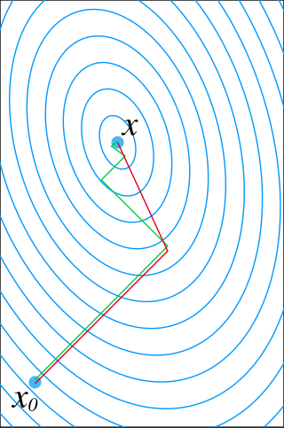
In mathematics, the conjugate gradient method is an algorithm for the numerical solution of particular systems of linear equations, namely those whose matrix is positive-semidefinite. The conjugate gradient method is often implemented as an iterative algorithm, applicable to sparse systems that are too large to be handled by a direct implementation or other direct methods such as the Cholesky decomposition. Large sparse systems often arise when numerically solving partial differential equations or optimization problems.
In differential geometry, a tensor density or relative tensor is a generalization of the tensor field concept. A tensor density transforms as a tensor field when passing from one coordinate system to another, except that it is additionally multiplied or weighted by a power W of the Jacobian determinant of the coordinate transition function or its absolute value. A tensor density with a single index is called a vector density. A distinction is made among (authentic) tensor densities, pseudotensor densities, even tensor densities and odd tensor densities. Sometimes tensor densities with a negative weight W are called tensor capacity. A tensor density can also be regarded as a section of the tensor product of a tensor bundle with a density bundle.

In statistics, simple linear regression (SLR) is a linear regression model with a single explanatory variable. That is, it concerns two-dimensional sample points with one independent variable and one dependent variable and finds a linear function that, as accurately as possible, predicts the dependent variable values as a function of the independent variable. The adjective simple refers to the fact that the outcome variable is related to a single predictor.
Methods of computing square roots are algorithms for approximating the non-negative square root of a positive real number . Since all square roots of natural numbers, other than of perfect squares, are irrational, square roots can usually only be computed to some finite precision: these methods typically construct a series of increasingly accurate approximations.
In statistics, a binomial proportion confidence interval is a confidence interval for the probability of success calculated from the outcome of a series of success–failure experiments. In other words, a binomial proportion confidence interval is an interval estimate of a success probability when only the number of experiments and the number of successes are known.

A pendulum is a body suspended from a fixed support so that it swings freely back and forth under the influence of gravity. When a pendulum is displaced sideways from its resting, equilibrium position, it is subject to a restoring force due to gravity that will accelerate it back towards the equilibrium position. When released, the restoring force acting on the pendulum's mass causes it to oscillate about the equilibrium position, swinging it back and forth. The mathematics of pendulums are in general quite complicated. Simplifying assumptions can be made, which in the case of a simple pendulum allow the equations of motion to be solved analytically for small-angle oscillations.
In numerical analysis, Aitken's delta-squared process or Aitken extrapolation is a series acceleration method, used for accelerating the rate of convergence of a sequence. It is named after Alexander Aitken, who introduced this method in 1926. Its early form was known to Seki Kōwa and was found for rectification of the circle, i.e. the calculation of π. It is most useful for accelerating the convergence of a sequence that is converging linearly.

In probability theory and statistics, the skew normal distribution is a continuous probability distribution that generalises the normal distribution to allow for non-zero skewness.
HyperLogLog is an algorithm for the count-distinct problem, approximating the number of distinct elements in a multiset. Calculating the exact cardinality of the distinct elements of a multiset requires an amount of memory proportional to the cardinality, which is impractical for very large data sets. Probabilistic cardinality estimators, such as the HyperLogLog algorithm, use significantly less memory than this, but can only approximate the cardinality. The HyperLogLog algorithm is able to estimate cardinalities of > 109 with a typical accuracy (standard error) of 2%, using 1.5 kB of memory. HyperLogLog is an extension of the earlier LogLog algorithm, itself deriving from the 1984 Flajolet–Martin algorithm.
(Stochastic) variance reduction is an algorithmic approach to minimizing functions that can be decomposed into finite sums. By exploiting the finite sum structure, variance reduction techniques are able to achieve convergence rates that are impossible to achieve with methods that treat the objective as an infinite sum, as in the classical Stochastic approximation setting.


