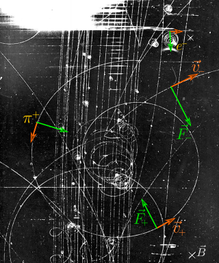
In physics, specifically in electromagnetism, the Lorentz force is the combination of electric and magnetic force on a point charge due to electromagnetic fields. A particle of charge q moving with a velocity v in an electric field E and a magnetic field B experiences a force of
In vector calculus and differential geometry the generalized Stokes theorem, also called the Stokes–Cartan theorem, is a statement about the integration of differential forms on manifolds, which both simplifies and generalizes several theorems from vector calculus. In particular, the fundamental theorem of calculus is the special case where the manifold is a line segment, Green’s theorem and Stokes' theorem are the cases of a surface in or and the divergence theorem is the case of a volume in Hence, the theorem is sometimes referred to as the Fundamental Theorem of Multivariate Calculus.

The Navier–Stokes equations are partial differential equations which describe the motion of viscous fluid substances. They were named after French engineer and physicist Claude-Louis Navier and the Irish physicist and mathematician George Gabriel Stokes. They were developed over several decades of progressively building the theories, from 1822 (Navier) to 1842–1850 (Stokes).
In physics, a Langevin equation is a stochastic differential equation describing how a system evolves when subjected to a combination of deterministic and fluctuating ("random") forces. The dependent variables in a Langevin equation typically are collective (macroscopic) variables changing only slowly in comparison to the other (microscopic) variables of the system. The fast (microscopic) variables are responsible for the stochastic nature of the Langevin equation. One application is to Brownian motion, which models the fluctuating motion of a small particle in a fluid.

In statistical mechanics and information theory, the Fokker–Planck equation is a partial differential equation that describes the time evolution of the probability density function of the velocity of a particle under the influence of drag forces and random forces, as in Brownian motion. The equation can be generalized to other observables as well. The Fokker-Planck equation has multiple applications in information theory, graph theory, data science, finance, economics etc.
The calculus of variations is a field of mathematical analysis that uses variations, which are small changes in functions and functionals, to find maxima and minima of functionals: mappings from a set of functions to the real numbers. Functionals are often expressed as definite integrals involving functions and their derivatives. Functions that maximize or minimize functionals may be found using the Euler–Lagrange equation of the calculus of variations.
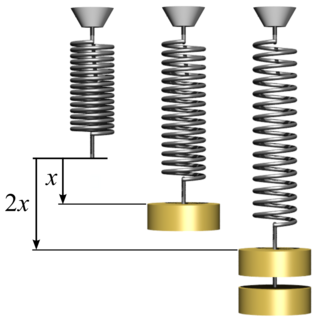
In physics, Hooke's law is an empirical law which states that the force needed to extend or compress a spring by some distance scales linearly with respect to that distance—that is, Fs = kx, where k is a constant factor characteristic of the spring, and x is small compared to the total possible deformation of the spring. The law is named after 17th-century British physicist Robert Hooke. He first stated the law in 1676 as a Latin anagram. He published the solution of his anagram in 1678 as: ut tensio, sic vis. Hooke states in the 1678 work that he was aware of the law since 1660.
A Newtonian fluid is a fluid in which the viscous stresses arising from its flow are at every point linearly correlated to the local strain rate — the rate of change of its deformation over time. Stresses are proportional to the rate of change of the fluid's velocity vector.

Stellar dynamics is the branch of astrophysics which describes in a statistical way the collective motions of stars subject to their mutual gravity. The essential difference from celestial mechanics is that the number of body
In physics and mathematics, the Helmholtz decomposition theorem or the fundamental theorem of vector calculus states that any sufficiently smooth, rapidly decaying vector field in three dimensions can be resolved into the sum of an irrotational (curl-free) vector field and a solenoidal (divergence-free) vector field. This is named after Hermann von Helmholtz.

In electromagnetism, charge density is the amount of electric charge per unit length, surface area, or volume. Volume charge density is the quantity of charge per unit volume, measured in the SI system in coulombs per cubic meter (C⋅m−3), at any point in a volume. Surface charge density (σ) is the quantity of charge per unit area, measured in coulombs per square meter (C⋅m−2), at any point on a surface charge distribution on a two dimensional surface. Linear charge density (λ) is the quantity of charge per unit length, measured in coulombs per meter (C⋅m−1), at any point on a line charge distribution. Charge density can be either positive or negative, since electric charge can be either positive or negative.

Toroidal coordinates are a three-dimensional orthogonal coordinate system that results from rotating the two-dimensional bipolar coordinate system about the axis that separates its two foci. Thus, the two foci and in bipolar coordinates become a ring of radius in the plane of the toroidal coordinate system; the -axis is the axis of rotation. The focal ring is also known as the reference circle.
There are various mathematical descriptions of the electromagnetic field that are used in the study of electromagnetism, one of the four fundamental interactions of nature. In this article, several approaches are discussed, although the equations are in terms of electric and magnetic fields, potentials, and charges with currents, generally speaking.
The derivation of the Navier–Stokes equations as well as its application and formulation for different families of fluids, is an important exercise in fluid dynamics with applications in mechanical engineering, physics, chemistry, heat transfer, and electrical engineering. A proof explaining the properties and bounds of the equations, such as Navier–Stokes existence and smoothness, is one of the important unsolved problems in mathematics.
In mathematics – specifically, in stochastic analysis – an Itô diffusion is a solution to a specific type of stochastic differential equation. That equation is similar to the Langevin equation used in physics to describe the Brownian motion of a particle subjected to a potential in a viscous fluid. Itô diffusions are named after the Japanese mathematician Kiyosi Itô.
The obstacle problem is a classic motivating example in the mathematical study of variational inequalities and free boundary problems. The problem is to find the equilibrium position of an elastic membrane whose boundary is held fixed, and which is constrained to lie above a given obstacle. It is deeply related to the study of minimal surfaces and the capacity of a set in potential theory as well. Applications include the study of fluid filtration in porous media, constrained heating, elasto-plasticity, optimal control, and financial mathematics.
Chapman–Enskog theory provides a framework in which equations of hydrodynamics for a gas can be derived from the Boltzmann equation. The technique justifies the otherwise phenomenological constitutive relations appearing in hydrodynamical descriptions such as the Navier–Stokes equations. In doing so, expressions for various transport coefficients such as thermal conductivity and viscosity are obtained in terms of molecular parameters. Thus, Chapman–Enskog theory constitutes an important step in the passage from a microscopic, particle-based description to a continuum hydrodynamical one.

Stokes' theorem, also known as the Kelvin–Stokes theorem after Lord Kelvin and George Stokes, the fundamental theorem for curls or simply the curl theorem, is a theorem in vector calculus on . Given a vector field, the theorem relates the integral of the curl of the vector field over some surface, to the line integral of the vector field around the boundary of the surface. The classical theorem of Stokes can be stated in one sentence: The line integral of a vector field over a loop is equal to the surface integral of its curl over the enclosed surface. It is illustrated in the figure, where the direction of positive circulation of the bounding contour ∂Σ, and the direction n of positive flux through the surface Σ, are related by a right-hand-rule. For the right hand the fingers circulate along ∂Σ and the thumb is directed along n.
Heat transfer physics describes the kinetics of energy storage, transport, and energy transformation by principal energy carriers: phonons, electrons, fluid particles, and photons. Heat is thermal energy stored in temperature-dependent motion of particles including electrons, atomic nuclei, individual atoms, and molecules. Heat is transferred to and from matter by the principal energy carriers. The state of energy stored within matter, or transported by the carriers, is described by a combination of classical and quantum statistical mechanics. The energy is different made (converted) among various carriers. The heat transfer processes are governed by the rates at which various related physical phenomena occur, such as the rate of particle collisions in classical mechanics. These various states and kinetics determine the heat transfer, i.e., the net rate of energy storage or transport. Governing these process from the atomic level to macroscale are the laws of thermodynamics, including conservation of energy.
Lagrangian field theory is a formalism in classical field theory. It is the field-theoretic analogue of Lagrangian mechanics. Lagrangian mechanics is used to analyze the motion of a system of discrete particles each with a finite number of degrees of freedom. Lagrangian field theory applies to continua and fields, which have an infinite number of degrees of freedom.


