Compositional data

Last updated February 03, 2024

In statistics, compositional data are quantitative descriptions of the parts of some whole, conveying relative information. Mathematically, compositional data is represented by points on a simplex. Measurements involving probabilities, proportions, percentages, and ppm can all be thought of as compositional data.

Ternary plot

Compositional data in three variables can be plotted via ternary plots. The use of a barycentric plot on three variables graphically depicts the ratios of the three variables as positions in an equilateral triangle.

Simplicial sample space

In general, John Aitchison defined compositional data to be proportions of some whole in 1982.^[1] In particular, a compositional data point (or composition for short) can be represented by a real vector with positive components. The sample space of compositional data is a simplex:

{\mathcal {S}}^{D}=\left\{\mathbf {x} =[x_{1},x_{2},\dots ,x_{D}]\in \mathbb {R} ^{D}\,\left|\,x_{i}>0,i=1,2,\dots ,D;\sum _{i=1}^{D}x_{i}=\kappa \right.\right\}.\

An illustration of the Aitchison simplex. Here, there are 3 parts,
x
1
,
x
2
,
x
3
{\displaystyle x_{1},x_{2},x_{3}}
represent values of different proportions. A, B, C, D and E are 5 different compositions within the simplex. A, B and C are all equivalent and D and E are equivalent. Aitchison-simplex.jpg — An illustration of the Aitchison simplex. Here, there are 3 parts, $x_{1},x_{2},x_{3}$ represent values of different proportions. A, B, C, D and E are 5 different compositions within the simplex. A, B and C are all equivalent and D and E are equivalent.

The only information is given by the ratios between components, so the information of a composition is preserved under multiplication by any positive constant. Therefore, the sample space of compositional data can always be assumed to be a standard simplex, i.e. $\kappa =1$ . In this context, normalization to the standard simplex is called closure and is denoted by $\scriptstyle {\mathcal {C}}[\,\cdot \,]$ :

{\mathcal {C}}[x_{1},x_{2},\dots ,x_{D}]=\left[{\frac {x_{1}}{\sum _{i=1}^{D}x_{i}}},{\frac {x_{2}}{\sum _{i=1}^{D}x_{i}}},\dots ,{\frac {x_{D}}{\sum _{i=1}^{D}x_{i}}}\right],\

where D is the number of parts (components) and $[\cdot ]$ denotes a row vector.

Aitchison geometry

The simplex can be given the structure of a real vector space in several different ways. The following vector space structure is called Aitchison geometry or the Aitchison simplex and has the following operations:

Perturbation

x\oplus y=\left[{\frac {x_{1}y_{1}}{\sum _{i=1}^{D}x_{i}y_{i}}},{\frac {x_{2}y_{2}}{\sum _{i=1}^{D}x_{i}y_{i}}},\dots ,{\frac {x_{D}y_{D}}{\sum _{i=1}^{D}x_{i}y_{i}}}\right]=C[x_{1}y_{1},\ldots ,x_{D}y_{D}]\qquad \forall x,y\in S^{D}

Powering

\alpha \odot x=\left[{\frac {x_{1}^{\alpha }}{\sum _{i=1}^{D}x_{i}^{\alpha }}},{\frac {x_{2}^{\alpha }}{\sum _{i=1}^{D}x_{i}^{\alpha }}},\ldots ,{\frac {x_{D}^{\alpha }}{\sum _{i=1}^{D}x_{i}^{\alpha }}}\right]=C[x_{1}^{\alpha },\ldots ,x_{D}^{\alpha }]\qquad \forall x\in S^{D},\;\alpha \in \mathbb {R}

Inner product

\langle x,y\rangle ={\frac {1}{2D}}\sum _{i=1}^{D}\sum _{j=1}^{D}\log {\frac {x_{i}}{x_{j}}}\log {\frac {y_{i}}{y_{j}}}\qquad \forall x,y\in S^{D}

Under these operations alone, it is sufficient to show that the Aitchison simplex forms a $(D-1)$ -dimensional Euclidean vector space.

Orthonormal bases

Since the Aitchison simplex forms a finite dimensional Hilbert space, it is possible to construct orthonormal bases in the simplex. Every composition $x$ can be decomposed as follows

x=\bigoplus _{i=1}^{D}x_{i}^{*}\odot e_{i}

where $e_{1},\ldots ,e_{D-1}$ forms an orthonormal basis in the simplex.^[2] The values $x_{i}^{*},i=1,2,\ldots ,D-1$ are the (orthonormal and Cartesian) coordinates of $x$ with respect to the given basis. They are called isometric log-ratio coordinates $(\operatorname {ilr} )$ .

Linear transformations

There are three well-characterized isomorphisms that transform from the Aitchison simplex to real space. All of these transforms satisfy linearity and as given below

Additive log ratio transform

The additive log ratio (alr) transform is an isomorphism where $\operatorname {alr} :S^{D}\rightarrow \mathbb {R} ^{D-1}$ . This is given by

\operatorname {alr} (x)=\left[\log {\frac {x_{1}}{x_{D}}}\cdots \log {\frac {x_{D-1}}{x_{D}}}\right]

The choice of denominator component is arbitrary, and could be any specified component. This transform is commonly used in chemistry with measurements such as pH. In addition, this is the transform most commonly used for multinomial logistic regression. The alr transform is not an isometry, meaning that distances on transformed values will not be equivalent to distances on the original compositions in the simplex.

Center log ratio transform

The center log ratio (clr) transform is both an isomorphism and an isometry where $\operatorname {clr} :S^{D}\rightarrow U,\quad U\subset \mathbb {R} ^{D}$

\operatorname {clr} (x)=\left[\log {\frac {x_{1}}{g(x)}}\cdots \log {\frac {x_{D}}{g(x)}}\right]

Where $g(x)$ is the geometric mean of $x$ . The inverse of this function is also known as the softmax function.

Isometric logratio transform

The isometric log ratio (ilr) transform is both an isomorphism and an isometry where $\operatorname {ilr} :S^{D}\rightarrow \mathbb {R} ^{D-1}$

\operatorname {ilr} (x)={\big [}\langle x,e_{1}\rangle ,\ldots ,\langle x,e_{D-1}\rangle {\big ]}

There are multiple ways to construct orthonormal bases, including using the Gram–Schmidt orthogonalization or singular-value decomposition of clr transformed data. Another alternative is to construct log contrasts from a bifurcating tree. If we are given a bifurcating tree, we can construct a basis from the internal nodes in the tree.

A representation of a tree in terms of its orthogonal components. l represents an internal node, an element of the orthonormal basis. This is a precursor to using the tree as a scaffold for the ilr transform Orthogonal-tree-basis.jpg — A representation of a tree in terms of its orthogonal components. l represents an internal node, an element of the orthonormal basis. This is a precursor to using the tree as a scaffold for the ilr transform

Each vector in the basis would be determined as follows

e_{\ell }=C[\exp(\,\underbrace {0,\ldots ,0} _{k},\underbrace {a,\ldots ,a} _{r},\underbrace {b,\ldots ,b} _{s},\underbrace {0,\ldots ,0} _{t}\,)]

The elements within each vector are given as follows

a={\frac {\sqrt {s}}{\sqrt {r(r+s)}}}\quad {\text{and}}\quad b={\frac {-{\sqrt {r}}}{\sqrt {s(r+s)}}}

where $k,r,s,t$ are the respective number of tips in the corresponding subtrees shown in the figure. It can be shown that the resulting basis is orthonormal^[3]

Once the basis $\Psi$ is built, the ilr transform can be calculated as follows

\operatorname {ilr} (x)=\operatorname {clr} (x)\Psi ^{T}

where each element in the ilr transformed data is of the following form

b_{i}={\sqrt {\frac {rs}{r+s}}}\log {\frac {g(x_{R})}{g(x_{S})}}

where $x_{R}$ and $x_{S}$ are the set of values corresponding to the tips in the subtrees $R$ and $S$

Examples

In chemistry, compositions can be expressed as molar concentrations of each component. As the sum of all concentrations is not determined, the whole composition of D parts is needed and thus expressed as a vector of D molar concentrations. These compositions can be translated into weight per cent multiplying each component by the appropriated constant.
In demography, a town may be a compositional data point in a sample of towns; a town in which 35% of the people are Christians, 55% are Muslims, 6% are Jews, and the remaining 4% are others would correspond to the quadruple [0.35, 0.55, 0.06, 0.04]. A data set would correspond to a list of towns.
In geology, a rock composed of different minerals may be a compositional data point in a sample of rocks; a rock of which 10% is the first mineral, 30% is the second, and the remaining 60% is the third would correspond to the triple [0.1, 0.3, 0.6]. A data set would contain one such triple for each rock in a sample of rocks.
In high throughput sequencing, data obtained are typically transformed to relative abundances, rendering them compositional.
In probability and statistics, a partition of the sampling space into disjoint events is described by the probabilities assigned to such events. The vector of D probabilities can be considered as a composition of D parts. As they add to one, one probability can be suppressed and the composition is completely determined.
In chemometrics, for the classification of petroleum oils.^[4]
In a survey, the proportions of people positively answering some different items can be expressed as percentages. As the total amount is identified as 100, the compositional vector of D components can be defined using only D − 1 components, assuming that the remaining component is the percentage needed for the whole vector to add to 100.

Notes

↑ Aitchison, John (1982). "The Statistical Analysis of Compositional Data". Journal of the Royal Statistical Society. Series B (Methodological). 44 (2): 139–177. doi:10.1111/j.2517-6161.1982.tb01195.x.
↑ Egozcue et al.
↑ Egozcue & Pawlowsky-Glahn 2005
↑ Olea, Ricardo A.; Martín-Fernández, Josep A.; Craddock, William H. (2021). "Multivariate classification of the crude oil petroleum systems in southeast Texas, USA, using conventional and compositional analysis of biomarkers". In Advances in Compositional Data Analysis—Festschrift in honor of Vera-Pawlowsky-Glahn, Filzmoser, P., Hron, K., Palarea-Albaladejo, J., Martín-Fernández, J.A., editors. Springer: 303−327.

Related Research Articles

In mathematics, the harmonic mean is one of several kinds of average, and in particular, one of the Pythagorean means. It is sometimes appropriate for situations when the average rate is desired.

In mathematics, an operator is generally a mapping or function that acts on elements of a space to produce elements of another space. There is no general definition of an operator, but the term is often used in place of function when the domain is a set of functions or other structured objects. Also, the domain of an operator is often difficult to characterize explicitly, and may be extended so as to act on related objects. See Operator (physics) for other examples.

In probability theory, the central limit theorem (CLT) states that, under appropriate conditions, the distribution of a normalized version of the sample mean converges to a standard normal distribution. This holds even if the original variables themselves are not normally distributed. There are several versions of the CLT, each applying in the context of different conditions.

<span class="mw-page-title-main">Simplex</span> Multi-dimensional generalization of triangle

In geometry, a simplex is a generalization of the notion of a triangle or tetrahedron to arbitrary dimensions. The simplex is so-named because it represents the simplest possible polytope in any given dimension. For example,

In statistics, maximum likelihood estimation (MLE) is a method of estimating the parameters of an assumed probability distribution, given some observed data. This is achieved by maximizing a likelihood function so that, under the assumed statistical model, the observed data is most probable. The point in the parameter space that maximizes the likelihood function is called the maximum likelihood estimate. The logic of maximum likelihood is both intuitive and flexible, and as such the method has become a dominant means of statistical inference.

In probability theory and statistics, the moment-generating function of a real-valued random variable is an alternative specification of its probability distribution. Thus, it provides the basis of an alternative route to analytical results compared with working directly with probability density functions or cumulative distribution functions. There are particularly simple results for the moment-generating functions of distributions defined by the weighted sums of random variables. However, not all random variables have moment-generating functions.

A discrete Hartley transform (DHT) is a Fourier-related transform of discrete, periodic data similar to the discrete Fourier transform (DFT), with analogous applications in signal processing and related fields. Its main distinction from the DFT is that it transforms real inputs to real outputs, with no intrinsic involvement of complex numbers. Just as the DFT is the discrete analogue of the continuous Fourier transform (FT), the DHT is the discrete analogue of the continuous Hartley transform (HT), introduced by Ralph V. L. Hartley in 1942.

In statistics, the Pearson correlation coefficient (PCC) is a correlation coefficient that measures linear correlation between two sets of data. It is the ratio between the covariance of two variables and the product of their standard deviations; thus, it is essentially a normalized measurement of the covariance, such that the result always has a value between −1 and 1. As with covariance itself, the measure can only reflect a linear correlation of variables, and ignores many other types of relationships or correlations. As a simple example, one would expect the age and height of a sample of teenagers from a high school to have a Pearson correlation coefficient significantly greater than 0, but less than 1.

In mathematics, a differential operator is an operator defined as a function of the differentiation operator. It is helpful, as a matter of notation first, to consider differentiation as an abstract operation that accepts a function and returns another function.

In probability theory, a compound Poisson distribution is the probability distribution of the sum of a number of independent identically-distributed random variables, where the number of terms to be added is itself a Poisson-distributed variable. The result can be either a continuous or a discrete distribution.

<span class="mw-page-title-main">Dirichlet distribution</span> Probability distribution

In probability and statistics, the Dirichlet distribution (after Peter Gustav Lejeune Dirichlet), often denoted $, is a family of continuous multivariate probability distributions parameterized by a vector of positive reals. It is a multivariate generalization of the beta distribution, hence its alternative name of multivariate beta distribution (MBD) . Dirichlet distributions are commonly used as prior distributions in Bayesian statistics, and in fact, the Dirichlet distribution is the conjugate prior of the categorical distribution and multinomial distribution.$

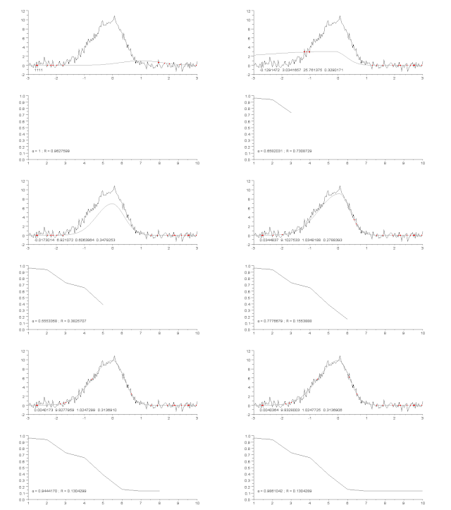
The Gauss–Newton algorithm is used to solve non-linear least squares problems, which is equivalent to minimizing a sum of squared function values. It is an extension of Newton's method for finding a minimum of a non-linear function. Since a sum of squares must be nonnegative, the algorithm can be viewed as using Newton's method to iteratively approximate zeroes of the components of the sum, and thus minimizing the sum. In this sense, the algorithm is also an effective method for solving overdetermined systems of equations. It has the advantage that second derivatives, which can be challenging to compute, are not required.

In statistics, Poisson regression is a generalized linear model form of regression analysis used to model count data and contingency tables. Poisson regression assumes the response variable Y has a Poisson distribution, and assumes the logarithm of its expected value can be modeled by a linear combination of unknown parameters. A Poisson regression model is sometimes known as a log-linear model, especially when used to model contingency tables.

A ratio distribution is a probability distribution constructed as the distribution of the ratio of random variables having two other known distributions. Given two random variables X and Y, the distribution of the random variable Z that is formed as the ratio Z = X/Y is a ratio distribution.

In probability theory and statistics, a categorical distribution is a discrete probability distribution that describes the possible results of a random variable that can take on one of K possible categories, with the probability of each category separately specified. There is no innate underlying ordering of these outcomes, but numerical labels are often attached for convenience in describing the distribution,. The K-dimensional categorical distribution is the most general distribution over a K-way event; any other discrete distribution over a size-K sample space is a special case. The parameters specifying the probabilities of each possible outcome are constrained only by the fact that each must be in the range 0 to 1, and all must sum to 1.

Non-linear least squares is the form of least squares analysis used to fit a set of m observations with a model that is non-linear in n unknown parameters (m ≥ n). It is used in some forms of nonlinear regression. The basis of the method is to approximate the model by a linear one and to refine the parameters by successive iterations. There are many similarities to linear least squares, but also some significant differences. In economic theory, the non-linear least squares method is applied in (i) the probit regression, (ii) threshold regression, (iii) smooth regression, (iv) logistic link regression, (v) Box–Cox transformed regressors ( $).$

In probability theory and statistics, the Poisson distribution is a discrete probability distribution that expresses the probability of a given number of events occurring in a fixed interval of time if these events occur with a known constant mean rate and independently of the time since the last event. It can also be used for the number of events in other types of intervals than time, and in dimension greater than 1.

Least-squares support-vector machines (LS-SVM) for statistics and in statistical modeling, are least-squares versions of support-vector machines (SVM), which are a set of related supervised learning methods that analyze data and recognize patterns, and which are used for classification and regression analysis. In this version one finds the solution by solving a set of linear equations instead of a convex quadratic programming (QP) problem for classical SVMs. Least-squares SVM classifiers were proposed by Johan Suykens and Joos Vandewalle. LS-SVMs are a class of kernel-based learning methods.

<span class="mw-page-title-main">Logit-normal distribution</span>

In probability theory, a logit-normal distribution is a probability distribution of a random variable whose logit has a normal distribution. If Y is a random variable with a normal distribution, and t is the standard logistic function, then X = t(Y) has a logit-normal distribution; likewise, if X is logit-normally distributed, then Y = logit(X)= log (X/(1-X)) is normally distributed. It is also known as the logistic normal distribution, which often refers to a multinomial logit version (e.g.).

The hyperbolastic functions, also known as hyperbolastic growth models, are mathematical functions that are used in medical statistical modeling. These models were originally developed to capture the growth dynamics of multicellular tumor spheres, and were introduced in 2005 by Mohammad Tabatabai, David Williams, and Zoran Bursac. The precision of hyperbolastic functions in modeling real world problems is somewhat due to their flexibility in their point of inflection. These functions can be used in a wide variety of modeling problems such as tumor growth, stem cell proliferation, pharma kinetics, cancer growth, sigmoid activation function in neural networks, and epidemiological disease progression or regression.

References

Aitchison, J. (2011) [1986], The Statistical Analysis of Compositional Data, Monographs on statistics and applied probability, Springer, ISBN 978-94-010-8324-9
van den Boogaart, K. Gerald; Tolosana-Delgado, Raimon (2013), Analyzing Compositional Data with R, Springer, ISBN 978-3-642-36809-7
Egozcue, Juan Jose; Pawlowsky-Glahn, Vera; Mateu-Figueras, Gloria; Barcelo-Vidal, Carles (2003), "Isometric logratio transformations for compositional data analysis", Mathematical Geology , 35 (3): 279–300, doi:10.1023/A:1023818214614, S2CID 122844634
Egozcue, Juan Jose; Pawlowsky-Glahn, Vera (2005), "Groups of parts and their balances in compositional data analysis", Mathematical Geology , 37 (7): 795–828, doi:10.1007/s11004-005-7381-9, S2CID 53061345
Pawlowsky-Glahn, Vera; Egozcue, Juan Jose; Tolosana-Delgado, Raimon (2015), Modeling and Analysis of Compositional Data, Wiley, doi:10.1002/9781119003144, ISBN 978-1-119-00314-4

External links

CoDaWeb – Compositional Data Website
Pawlowsky-Glahn, V.; Egozcue, J.J.; Tolosana-Delgado, R. (2007). "Lecture Notes on Compositional Data Analysis". Universitat de Girona. hdl: 10256/297 .
Why, and How, Should Geologists Use Compositional Data Analysis (wikibook)

This page is based on this Wikipedia article
Text is available under the CC BY-SA 4.0 license; additional terms may apply.
Images, videos and audio are available under their respective licenses.

[1] Aitchison, John (1982). "The Statistical Analysis of Compositional Data". Journal of the Royal Statistical Society. Series B (Methodological). 44 (2): 139–177. doi:10.1111/j.2517-6161.1982.tb01195.x.

[2] Egozcue et al.

[3] Egozcue & Pawlowsky-Glahn 2005

[4] Olea, Ricardo A.; Martín-Fernández, Josep A.; Craddock, William H. (2021). "Multivariate classification of the crude oil petroleum systems in southeast Texas, USA, using conventional and compositional analysis of biomarkers". In Advances in Compositional Data Analysis—Festschrift in honor of Vera-Pawlowsky-Glahn, Filzmoser, P., Hron, K., Palarea-Albaladejo, J., Martín-Fernández, J.A., editors. Springer: 303−327.

[1]

[2]

[3]

[4]