
In economics, profit maximization is the short run or long run process by which a firm may determine the price, input and output levels that lead to the highest profit. Neoclassical economics, currently the mainstream approach to microeconomics, usually models the firm as maximizing profit.
The following outline is provided as an overview of and topical guide to industrial organization:
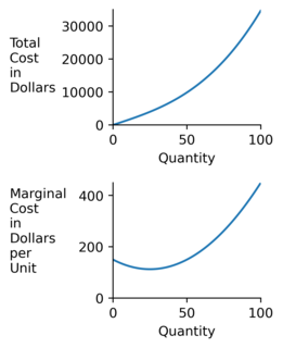
In economics, the marginal cost is the change in the total cost that arises when the quantity produced is incremented, the cost of producing additional quantity. In some contexts, it refers to an increment of one unit of output, and in others it refers to the rate of change of total cost as output is increased by an infinitesimal amount. As Figure 1 shows, the marginal cost is measured in dollars per unit, whereas total cost is in dollars, and the marginal cost is the slope of the total cost, the rate at which it increases with output. Marginal cost is different from average cost, which is the total cost divided by the number of units produced.

In economics, a production function gives the technological relation between quantities of physical inputs and quantities of output of goods. The production function is one of the key concepts of mainstream neoclassical theories, used to define marginal product and to distinguish allocative efficiency, a key focus of economics. One important purpose of the production function is to address allocative efficiency in the use of factor inputs in production and the resulting distribution of income to those factors, while abstracting away from the technological problems of achieving technical efficiency, as an engineer or professional manager might understand it.
In economics, aggregate supply (AS) or domestic final supply (DFS) is the total supply of goods and services that firms in a national economy plan on selling during a specific time period. It is the total amount of goods and services that firms are willing and able to sell at a given price level in an economy.

In economics and in particular neoclassical economics, the marginal product or marginal physical productivity of an input is the change in output resulting from employing one more unit of a particular input, assuming that the quantities of other inputs are kept constant.

In economics, diminishing returns is the decrease in marginal (incremental) output of a production process as the amount of a single factor of production is incrementally increased, holding all other factors of production equal. The law of diminishing returns states that in productive processes, increasing a factor of production by one unit, while holding all others production factors constant, will at some point return a lower unit of output per incremental unit of input. The law of diminishing returns does not cause a decrease in overall production capabilities, rather it defines a point on a production curve whereby producing an additional unit of output will result in a loss and is known as negative returns. Under diminishing returns, output remains positive however productivity and efficiency decrease.
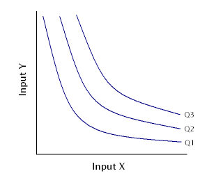
An isoquant, in microeconomics, is a contour line drawn through the set of points at which the same quantity of output is produced while changing the quantities of two or more inputs. The x and y axis on an isoquant represent two relevant inputs, which are usually a factor of production such as labour, capital, land, or organisation. An isoquant may also be known as an “Iso-Product Curve”, or an “Equal Product Curve”.
In economics, returns to scale describe what happens to long run returns as the scale of production increases, when all input levels including physical capital usage are variable. The concept of returns to scale arises in the context of a firm's production function. It explains the long run linkage of the rate of increase in output (production) relative to associated increases in the inputs. In the long run, all factors of production are variable and subject to change in response to a given increase in production scale. While economies of scale show the effect of an increased output level on unit costs, returns to scale focus only on the relation between input and output quantities.

In economics an isocost line shows all combinations of inputs which cost the same total amount. Although similar to the budget constraint in consumer theory, the use of the isocost line pertains to cost-minimization in production, as opposed to utility-maximization. For the two production inputs labour and capital, with fixed unit costs of the inputs, the equation of the isocost line is
In economics, a cost curve is a graph of the costs of production as a function of total quantity produced. In a free market economy, productively efficient firms optimize their production process by minimizing cost consistent with each possible level of production, and the result is a cost curve. Profit-maximizing firms use cost curves to decide output quantities. There are various types of cost curves, all related to each other, including total and average cost curves; marginal cost curves, which are equal to the differential of the total cost curves; and variable cost curves. Some are applicable to the short run, others to the long run.

In economics, total cost (TC) is the minimum dollar cost of producing some quantity of output. This is the total economic cost of production and is made up of variable cost, which varies according to the quantity of a good produced and includes inputs such as labor and raw materials, plus fixed cost, which is independent of the quantity of a good produced and includes inputs that cannot be varied in the short term such as buildings and machinery, including possibly sunk costs.
In economics the long-run is a theoretical concept in which all markets are in equilibrium, and all prices and quantities have fully adjusted and are in equilibrium. The long-run contrasts with the short-run, in which there are some constraints and markets are not fully in equilibrium.
In microeconomic theory, the marginal rate of technical substitution (MRTS)—or technical rate of substitution (TRS)—is the amount by which the quantity of one input has to be reduced when one extra unit of another input is used, so that output remains constant.
In economics, supply is the amount of a resource that firms, producers, labourers, providers of financial assets, or other economic agents are willing and able to provide to the marketplace or to an individual. Supply can be in produced goods, labor time, raw materials, or any other scarce or valuable object. Supply is often plotted graphically as a supply curve, with the price per unit on the vertical axis and quantity supplied as a function of price on the horizontal axis. This reversal of the usual position of the dependent variable and the independent variable is an unfortunate but standard convention.
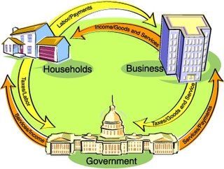
In economics, factor payments are the income people receive for supplying the factors of production: land, labor, capital or entrepreneurship.
In economics, the marginal product of labor (MPL) is the change in output that results from employing an added unit of labor. It is a feature of the production function, and depends on the amounts of physical capital and labor already in use.
In economics, the labor demand of an employer is the number of labor-hours that the employer is willing to hire based on the various exogenous variables it is faced with, such as the wage rate, the unit cost of capital, the market-determined selling price of its output, etc. The function specifying the quantity of labor that would be demanded at any of various possible values of these exogenous variables is called the labor demand function. The sum of the labor-hours demanded by all employers in total is the market demand for labor.
The Fei–Ranis model of economic growth is a dualism model in developmental economics or welfare economics that has been developed by John C. H. Fei and Gustav Ranis and can be understood as an extension of the Lewis model. It is also known as the Surplus Labor model. It recognizes the presence of a dual economy comprising both the modern and the primitive sector and takes the economic situation of unemployment and underemployment of resources into account, unlike many other growth models that consider underdeveloped countries to be homogenous in nature. According to this theory, the primitive sector consists of the existing agricultural sector in the economy, and the modern sector is the rapidly emerging but small industrial sector. Both the sectors co-exist in the economy, wherein lies the crux of the development problem. Development can be brought about only by a complete shift in the focal point of progress from the agricultural to the industrial economy, such that there is augmentation of industrial output. This is done by transfer of labor from the agricultural sector to the industrial one, showing that underdeveloped countries do not suffer from constraints of labor supply. At the same time, growth in the agricultural sector must not be negligible and its output should be sufficient to support the whole economy with food and raw materials. Like in the Harrod–Domar model, saving and investment become the driving forces when it comes to economic development of underdeveloped countries.
In economics, an expansion path is a path connecting optimal input combinations as the scale of production expands. which is often represented as a curve in a graph with quantities of two inputs, typically physical capital and labor, plotted on the axes. A producer seeking to produce a given number of units of a product in the cheapest possible way chooses the point on the expansion path that is also on the isoquant associated with that output level.


