Configuration (polytope)

Last updated

In geometry, H. S. M. Coxeter called a regular polytope a special kind of configuration.

Contents

Other configurations in geometry are something different. These polytope configurations may be more accurately called incidence matrices, where like elements are collected together in rows and columns. Regular polytopes will have one row and column per k-face element, while other polytopes will have one row and column for each k-face type by their symmetry classes. A polytope with no symmetry will have one row and column for every element, and the matrix will be filled with 0 if the elements are not connected, and 1 if they are connected. Elements of the same k will not be connected and will have a "*" table entry. [1]

Every polytope, and abstract polytope has a Hasse diagram expressing these connectivities, which can be systematically described with an incidence matrix.

Configuration matrix for regular polytopes

A configuration for a regular polytope is represented by a matrix where the diagonal element, Ni, is the number of i-faces in the polytope. The diagonal elements are also called a polytope's f-vector. The nondiagonal (ij) element Nij is the number of j-faces incident with each i-face element, so that NiNij = NjNji. [2]

The principle extends generally to n dimensions, where 0 ≤ j < n.

Polygons

A regular polygon, Schläfli symbol {q}, will have a 2x2 matrix, with the first row for vertices, and second row for edges. The order  g is 2q.

A general n-gon will have a 2n x 2n matrix, with the first n rows and columns vertices, and the last n rows and columns as edges.

Triangle example

There are three symmetry classifications of a triangle: equilateral, isosceles, and scalene. They all have the same incidence matrix, but symmetry allows vertices and edges to be collected together and counted. These triangles have vertices labeled A,B,C, and edges a,b,c, while vertices and edges that can be mapped onto each other by a symmetry operation are labeled identically.

Triangles
Equilateral
{3}
Equilateral triangle element-labeled.png
Isosceles
{ }∨( )
Isos triangle element-labeled.png
Scalene
( )∨( )∨( )
Scalene triangle element-labeled.png
(v:3; e:3)(v:2+1; e:2+1)(v:1+1+1; e:1+1+1)
  | A | a  --+---+--- A | 3 | 2  --+---+--- a | 2 | 3  
  | A B | a b --+-----+----- A | 2 * | 1 1 B | * 1 | 2 0 --+-----+----- a | 1 1 | 2 *  b | 2 0 | * 1  
  | A B C | a b c --+-------+------- A | 1 * * | 0 1 1 B | * 1 * | 1 0 1  C | * * 1 | 1 1 0  --+-------+------- a | 0 1 1 | 1 * *  b | 1 0 1 | * 1 *  c | 1 1 0 | * * 1 

Quadrilaterals

Quadrilaterals by symmetry Symmetries of square.svg
Quadrilaterals by symmetry

Quadrilaterals can be classified by symmetry, each with their own matrix. Quadrilaterals exist with dual pairs which will have the same matrix, rotated 180 degrees, with vertices and edges reversed. Squares and parallelograms, and general quadrilaterals are self-dual by class so their matrices are unchanged when rotated 180 degrees.

Quadrilaterals
Square
{4}
Square element-labeled.png
Rectangle
{ }×{ }
Rectangle element-labeled.png
Rhombus
{ }+{ }
Rhombus element-labeled.png
Parallelogram
Parallelogram element-labeled.png
(v:4; e:4)(v:4; e:2+2)(v:2+2; e:4)(v:2+2; e:2+2)
  | A | a  --+---+--- A | 4 | 2  --+---+--- a | 2 | 4 
  | A | a b --+---+----- A | 4 | 1 1 --+---+----- a | 2 | 2 *  b | 2 | * 2  
  | A B | a --+-----+--- A | 2 * | 2  B | * 2 | 2  --+-----+--- a | 1 1 | 4 
  | A B | a b --+-----+----- A | 2 * | 1 1 B | * 2 | 1 1 --+-----+----- a | 1 1 | 2 *  b | 1 1 | * 2  
Isosceles trapezoid
{ }||{ }
Isos trapezoid element-labeled.png
Kite
Kite element-labeled.png
General
Quadrilateral element-labeled.png
(v:2+2; e:1+1+2)(v:1+1+2; e:2+2)(v:1+1+1+1; e:1+1+1+1)
  | A B | a b c --+-----+------- A | 2 * | 1 0 1  B | * 2 | 0 1 1 --+-----+------ a | 2 0 | 1 * * b | 0 2 | * 1 * c | 1 1 | * * 2  
  | A B C | a b --+-------+---- A | 1 * * | 2 0  B | * 1 * | 0 2 C | * * 2 | 1 1 --+-------+---- a | 1 0 1 | 2 * b | 0 1 1 | * 2  
  | A B C D | a b c d --+---------+-------- A | 1 * * * | 1 0 0 1 B | * 1 * * | 1 1 0 0  C | * * 1 * | 0 1 1 0 D | * * * 1 | 0 0 1 1 --+---------+-------- a | 1 1 0 0 | 1 * * * b | 0 1 1 0 | * 1 * * c | 0 0 1 1 | * * 1 * d | 1 0 0 1 | * * * 1  

Complex polygons

The idea is also applicable for regular complex polygons, p{q}r constructed in :

The complex reflection group is p[q]r, order . [3] [4]

Polyhedra

The idea can be applied in three dimensions by considering incidences of points, lines and planes, or j-spaces (0 ≤ j < 3), where each j-space is incident with Njkk-spaces (jk). Writing Nj for the number of j-spaces present, a given configuration may be represented by the matrix

for Schläfli symbol {p,q}, with group order  g = 4pq/(4  (p  2)(q  2)).

Tetrahedron

Symmetries of tetrahedra Tetrahedron symmetry tree.png
Symmetries of tetrahedra

Tetrahedra have matrices that can also be grouped by their symmetry, with a general tetrahedron having 14 rows and columns for the 4 vertices, 6 edges, and 4 faces. Tetrahedra are self-dual, and rotating the matices 180 degrees (swapping vertices and faces) will leave it unchanged.

Tetrahedra
Regular
(v:4; e:6; f:4)
Tetrahedron type1.png
tetragonal disphenoid
(v:4; e:2+4; f:4)
Tetrahedron type2.png
Rhombic disphenoid
(v:4; e:2+2+2; f:4)
Tetrahedron type3.png
Digonal disphenoid
(v:2+2; e:4+1+1; f:2+2)
Tetrahedron type6.png
Phyllic disphenoid
(v:2+2; e:2+2+1+1; f:2+2)
Tetrahedron type4.png
  A| 4 | 3 | 3 ---+---+---+--   a| 2 | 6 | 2 ---+---+---+-- aaa| 3 | 3 | 4 
  A| 4 | 2 1 | 3 ---+---+-----+--   a| 2 | 4 * | 2   b| 2 | * 2 | 2 ---+---+-----+-- aab| 3 | 2 1 | 4 
   A| 4 | 1 1 1 | 3 ----+---+-------+--    a| 2 | 2 * * | 2    b| 2 | * 2 * | 2    c| 2 | * * 2 | 2 ----+---+-------+--  abc| 3 | 1 1 1 | 4 
  A| 2 * | 2 1 0 | 2 1   B| * 2 | 2 0 1 | 1 2 ---+-----+-------+----   a| 1 1 | 4 * * | 1 1   b| 2 0 | * 1 * | 2 0   c| 0 2 | * * 1 | 0 2 ---+-----+-------+---- aab| 2 1 | 2 1 0 | 2 * aac| 1 2 | 2 0 1 | * 2 
  A| 2 * | 1 0 1 1 | 1 2   B| * 2 | 1 1 1 0 | 2 1 ---+-----+---------+----   a| 1 1 | 2 * * * | 1 1   b| 1 1 | * 2 * * | 1 1   c| 0 2 | * * 1 * | 2 0   d| 2 0 | * * * 1 | 0 2 ---+-----+---------+---- abc| 1 2 | 1 1 1 0 | 2 * bcd| 2 1 | 1 1 0 1 | * 2 
Triangular pyramid
(v:3+1; e:3+3; f:3+1)
Tetrahedron type5.png
Mirrored spheroid
(v:2+1+1; e:2+2+1+1; f:2+1+1)
Tetrahedron type7.png
No symmetry
(v:1+1+1+1; e:1+1+1+1+1+1; f:1+1+1+1)
Tetrahedron type8.png
  A| 3 * | 2 1 | 2 1   B| * 1 | 0 3 | 3 0 ---+-----+-----+----   a| 2 0 | 3 * | 1 1   b| 1 1 | * 3 | 2 0 ---+-----+-----+---- abb| 2 1 | 1 2 | 3 * aaa| 3 0 | 3 0 | * 1 
  A| 2 * * | 1 1 0 1 | 1 1 1    B| * 1 * | 2 0 1 0 | 0 2 1    C| * * 1 | 0 2 1 0 | 1 2 0  ---+-------+---------+------   a| 1 0 1 | 2 * * * | 0 1 1    b| 0 1 1 | * 2 * * | 1 1 0    c| 1 1 0 | * * 1 * | 0 2 0    d| 0 0 2 | * * * 1 | 1 0 1  ---+-------+---------+------ ABC| 1 1 1 | 1 1 1 0 | 2 * * ACC| 1 0 2 | 2 0 0 1 | * 1 * BCC| 0 1 2 | 0 2 0 1 | * * 1 
  A | 1 0 0 0 | 1 1 1 0 0 0 | 1 1 1 0   B | 0 1 0 0 | 1 0 0 1 1 0 | 1 1 0 1   C | 0 0 1 0 | 0 1 0 1 0 1 | 1 0 1 1   D | 0 0 0 1 | 0 0 1 0 1 1 | 0 1 1 1 ----+---------+-------------+--------   a | 1 1 0 0 | 1 0 0 0 0 0 | 1 1 0 0   b | 1 0 1 0 | 0 1 0 0 0 0 | 1 0 1 0   c | 1 0 0 1 | 0 0 1 0 0 0 | 0 1 1 0   d | 0 1 1 0 | 0 0 0 1 0 0 | 1 0 0 1   e | 0 1 0 1 | 0 0 0 0 1 0 | 0 1 0 1   f | 0 0 1 1 | 0 0 0 0 0 1 | 0 0 1 1 ----+---------+-------------+-------- ABC | 1 1 1 0 | 1 1 0 1 0 0 | 1 0 0 0 ABD | 1 1 0 1 | 1 0 1 0 1 0 | 0 1 0 0 ACD | 1 0 1 1 | 0 1 1 0 0 1 | 0 0 1 0 BCD | 0 1 1 1 | 0 0 0 1 1 1 | 0 0 0 1

Notes

  1. Klitzing, Richard. "Incidence Matrices".
  2. Coxeter, Complex Regular Polytopes, p. 117
  3. Lehrer & Taylor 2009, p.87
  4. Complex Regular Polytopes, p. 117

Related Research Articles

<span class="mw-page-title-main">Cube</span> Solid object with six equal square faces

In geometry, a cube is a three-dimensional solid object bounded by six square faces, facets, or sides, with three meeting at each vertex. Viewed from a corner, it is a hexagon and its net is usually depicted as a cross.

<span class="mw-page-title-main">Matrix multiplication</span> Mathematical operation in linear algebra

In mathematics, particularly in linear algebra, matrix multiplication is a binary operation that produces a matrix from two matrices. For matrix multiplication, the number of columns in the first matrix must be equal to the number of rows in the second matrix. The resulting matrix, known as the matrix product, has the number of rows of the first and the number of columns of the second matrix. The product of matrices A and B is denoted as AB.

In mathematics, an incidence matrix is a logical matrix that shows the relationship between two classes of objects, usually called an incidence relation. If the first class is X and the second is Y, the matrix has one row for each element of X and one column for each element of Y. The entry in row x and column y is 1 if x and y are related and 0 if they are not. There are variations; see below.

In mathematics, a block matrix or a partitioned matrix is a matrix that is interpreted as having been broken into sections called blocks or submatrices. Intuitively, a matrix interpreted as a block matrix can be visualized as the original matrix with a collection of horizontal and vertical lines, which break it up, or partition it, into a collection of smaller matrices. Any matrix may be interpreted as a block matrix in one or more ways, with each interpretation defined by how its rows and columns are partitioned.

In the mathematical field of graph theory, Kirchhoff's theorem or Kirchhoff's matrix tree theorem named after Gustav Kirchhoff is a theorem about the number of spanning trees in a graph, showing that this number can be computed in polynomial time from the determinant of a submatrix of the Laplacian matrix of the graph; specifically, the number is equal to any cofactor of the Laplacian matrix. Kirchhoff's theorem is a generalization of Cayley's formula which provides the number of spanning trees in a complete graph.

In mathematics, a Coxeter element is an element of an irreducible Coxeter group which is a product of all simple reflections. The product depends on the order in which they are taken, but different orderings produce conjugate elements, which have the same order. This order is known as the Coxeter number. They are named after British-Canadian geometer H.S.M. Coxeter, who introduced the groups in 1934 as abstractions of reflection groups.

In five-dimensional geometry, a 5-cube is a name for a five-dimensional hypercube with 32 vertices, 80 edges, 80 square faces, 40 cubic cells, and 10 tesseract 4-faces.

<span class="mw-page-title-main">5-orthoplex</span>

In five-dimensional geometry, a 5-orthoplex, or 5-cross polytope, is a five-dimensional polytope with 10 vertices, 40 edges, 80 triangle faces, 80 tetrahedron cells, 32 5-cell 4-faces.

In geometry, a quasiregular polyhedron is a uniform polyhedron that has exactly two kinds of regular faces, which alternate around each vertex. They are vertex-transitive and edge-transitive, hence a step closer to regular polyhedra than the semiregular, which are merely vertex-transitive.

In five-dimensional geometry, a 5-simplex is a self-dual regular 5-polytope. It has six vertices, 15 edges, 20 triangle faces, 15 tetrahedral cells, and 6 5-cell facets. It has a dihedral angle of cos−1(1/5), or approximately 78.46°.

<span class="mw-page-title-main">6-cube</span> 6-dimensional hypercube

In geometry, a 6-cube is a six-dimensional hypercube with 64 vertices, 192 edges, 240 square faces, 160 cubic cells, 60 tesseract 4-faces, and 12 5-cube 5-faces.

<span class="mw-page-title-main">6-orthoplex</span>

In geometry, a 6-orthoplex, or 6-cross polytope, is a regular 6-polytope with 12 vertices, 60 edges, 160 triangle faces, 240 tetrahedron cells, 192 5-cell 4-faces, and 64 5-faces.

<span class="mw-page-title-main">7-cube</span> 7-dimensional hypercube

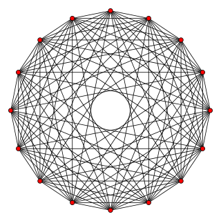
In geometry, a 7-cube is a seven-dimensional hypercube with 128 vertices, 448 edges, 672 square faces, 560 cubic cells, 280 tesseract 4-faces, 84 penteract 5-faces, and 14 hexeract 6-faces.

<span class="mw-page-title-main">8-cube</span> 8-dimensional hypercube

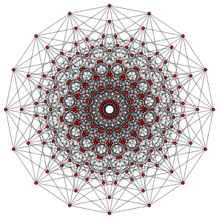
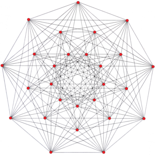
In geometry, an 8-cube is an eight-dimensional hypercube. It has 256 vertices, 1024 edges, 1792 square faces, 1792 cubic cells, 1120 tesseract 4-faces, 448 5-cube 5-faces, 112 6-cube 6-faces, and 16 7-cube 7-faces.

<span class="mw-page-title-main">7-orthoplex</span>

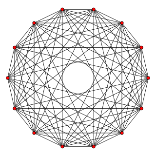
In geometry, a 7-orthoplex, or 7-cross polytope, is a regular 7-polytope with 14 vertices, 84 edges, 280 triangle faces, 560 tetrahedron cells, 672 5-cells 4-faces, 448 5-faces, and 128 6-faces.

In geometry, a 6-simplex is a self-dual regular 6-polytope. It has 7 vertices, 21 edges, 35 triangle faces, 35 tetrahedral cells, 21 5-cell 4-faces, and 7 5-simplex 5-faces. Its dihedral angle is cos−1(1/6), or approximately 80.41°.

<span class="mw-page-title-main">7-simplex</span>

In 7-dimensional geometry, a 7-simplex is a self-dual regular 7-polytope. It has 8 vertices, 28 edges, 56 triangle faces, 70 tetrahedral cells, 56 5-cell 5-faces, 28 5-simplex 6-faces, and 8 6-simplex 7-faces. Its dihedral angle is cos−1(1/7), or approximately 81.79°.

<span class="mw-page-title-main">8-orthoplex</span>

In geometry, an 8-orthoplex or 8-cross polytope is a regular 8-polytope with 16 vertices, 112 edges, 448 triangle faces, 1120 tetrahedron cells, 1792 5-cells 4-faces, 1792 5-faces, 1024 6-faces, and 256 7-faces.

<span class="mw-page-title-main">8-simplex</span>

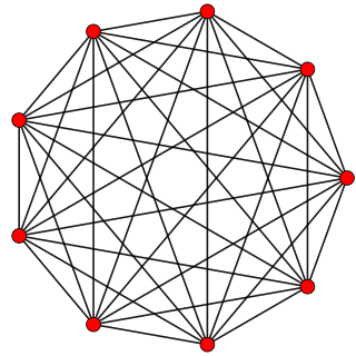
In geometry, an 8-simplex is a self-dual regular 8-polytope. It has 9 vertices, 36 edges, 84 triangle faces, 126 tetrahedral cells, 126 5-cell 4-faces, 84 5-simplex 5-faces, 36 6-simplex 6-faces, and 9 7-simplex 7-faces. Its dihedral angle is cos−1(1/8), or approximately 82.82°.

<span class="mw-page-title-main">Hessian polyhedron</span>

In geometry, the Hessian polyhedron is a regular complex polyhedron 3{3}3{3}3, , in . It has 27 vertices, 72 3{} edges, and 27 3{3}3 faces. It is self-dual.

References