In mathematics, Gaussian elimination, also known as row reduction, is an algorithm for solving systems of linear equations. It consists of a sequence of operations performed on the corresponding matrix of coefficients. This method can also be used to compute the rank of a matrix, the determinant of a square matrix, and the inverse of an invertible matrix. The method is named after Carl Friedrich Gauss (1777–1855) although some special cases of the method—albeit presented without proof—were known to Chinese mathematicians as early as circa 179 CE.

In combinatorics and in experimental design, a Latin square is an n × n array filled with n different symbols, each occurring exactly once in each row and exactly once in each column. An example of a 3×3 Latin square is
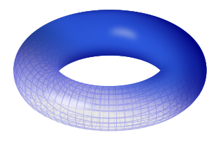
In geometry, a torus is a surface of revolution generated by revolving a circle in three-dimensional space about an axis that is coplanar with the circle.

In mathematics, particularly in linear algebra, matrix multiplication is a binary operation that produces a matrix from two matrices. For matrix multiplication, the number of columns in the first matrix must be equal to the number of rows in the second matrix. The resulting matrix, known as the matrix product, has the number of rows of the first and the number of columns of the second matrix. The product of matrices A and B is denoted as AB.

In numerical analysis and scientific computing, a sparse matrix or sparse array is a matrix in which most of the elements are zero. There is no strict definition regarding the proportion of zero-value elements for a matrix to qualify as sparse but a common criterion is that the number of non-zero elements is roughly equal to the number of rows or columns. By contrast, if most of the elements are non-zero, the matrix is considered dense. The number of zero-valued elements divided by the total number of elements is sometimes referred to as the sparsity of the matrix.
In combinatorics, two Latin squares of the same size (order) are said to be orthogonal if when superimposed the ordered paired entries in the positions are all distinct. A set of Latin squares, all of the same order, all pairs of which are orthogonal is called a set of mutually orthogonal Latin squares. This concept of orthogonality in combinatorics is strongly related to the concept of blocking in statistics, which ensures that independent variables are truly independent with no hidden confounding correlations. "Orthogonal" is thus synonymous with "independent" in that knowing one variable's value gives no further information about another variable's likely value.
In mathematics, a Hadamard matrix, named after the French mathematician Jacques Hadamard, is a square matrix whose entries are either +1 or −1 and whose rows are mutually orthogonal. In geometric terms, this means that each pair of rows in a Hadamard matrix represents two perpendicular vectors, while in combinatorial terms, it means that each pair of rows has matching entries in exactly half of their columns and mismatched entries in the remaining columns. It is a consequence of this definition that the corresponding properties hold for columns as well as rows. The n-dimensional parallelotope spanned by the rows of an n×n Hadamard matrix has the maximum possible n-dimensional volume among parallelotopes spanned by vectors whose entries are bounded in absolute value by 1. Equivalently, a Hadamard matrix has maximal determinant among matrices with entries of absolute value less than or equal to 1 and so is an extremal solution of Hadamard's maximal determinant problem.
In mathematics, a unimodular matrixM is a square integer matrix having determinant +1 or −1. Equivalently, it is an integer matrix that is invertible over the integers: there is an integer matrix N that is its inverse. Thus every equation Mx = b, where M and b both have integer components and M is unimodular, has an integer solution. The n × n unimodular matrices form a group called the n × n general linear group over , which is denoted .
In mathematics, computer science and especially graph theory, a distance matrix is a square matrix containing the distances, taken pairwise, between the elements of a set. Depending upon the application involved, the distance being used to define this matrix may or may not be a metric. If there are N elements, this matrix will have size N×N. In graph-theoretic applications the elements are more often referred to as points, nodes or vertices.

In combinatorial mathematics, a de Bruijn sequence of order n on a size-k alphabet A is a cyclic sequence in which every possible length-n string on A occurs exactly once as a substring. Such a sequence is denoted by B(k, n) and has length kn, which is also the number of distinct strings of length n on A. Each of these distinct strings, when taken as a substring of B(k, n), must start at a different position, because substrings starting at the same position are not distinct. Therefore, B(k, n) must have at leastkn symbols. And since B(k, n) has exactlykn symbols, De Bruijn sequences are optimally short with respect to the property of containing every string of length n at least once.
Combinatorial design theory is the part of combinatorial mathematics that deals with the existence, construction and properties of systems of finite sets whose arrangements satisfy generalized concepts of balance and/or symmetry. These concepts are not made precise so that a wide range of objects can be thought of as being under the same umbrella. At times this might involve the numerical sizes of set intersections as in block designs, while at other times it could involve the spatial arrangement of entries in an array as in sudoku grids.
A logical matrix, binary matrix, relation matrix, Boolean matrix, or (0, 1) matrix is a matrix with entries from the Boolean domain B = {0, 1}. Such a matrix can be used to represent a binary relation between a pair of finite sets.
In mathematics, a conference matrix is a square matrix C with 0 on the diagonal and +1 and −1 off the diagonal, such that CTC is a multiple of the identity matrix I. Thus, if the matrix has order n, CTC = (n−1)I. Some authors use a more general definition, which requires there to be a single 0 in each row and column but not necessarily on the diagonal.
In mathematics, particularly matrix theory and combinatorics, a Pascal matrix is a matrix containing the binomial coefficients as its elements. It is thus an encoding of Pascal's triangle in matrix form. There are three natural ways to achieve this: as a lower-triangular matrix, an upper-triangular matrix, or a symmetric matrix. For example, the 5 × 5 matrices are:
In mathematics a regular Hadamard matrix is a Hadamard matrix whose row and column sums are all equal. While the order of a Hadamard matrix must be 1, 2, or a multiple of 4, regular Hadamard matrices carry the further restriction that the order be a square number. The excess, denoted E(H), of a Hadamard matrix H of order n is defined to be the sum of the entries of H. The excess satisfies the bound |E(H)| ≤ n3/2. A Hadamard matrix attains this bound if and only if it is regular.

In mathematics, a matrix is a rectangular array or table of numbers, symbols, or expressions, arranged in rows and columns, which is used to represent a mathematical object or a property of such an object.
In discrete mathematics, the Bregman–Minc inequality, or Bregman's theorem, allows one to estimate the permanent of a binary matrix via its row or column sums. The inequality was conjectured in 1963 by Henryk Minc and first proved in 1973 by Lev M. Bregman. Further entropy-based proofs have been given by Alexander Schrijver and Jaikumar Radhakrishnan. The Bregman–Minc inequality is used, for example, in graph theory to obtain upper bounds for the number of perfect matchings in a bipartite graph.

In number theory, the Moser–De Bruijn sequence is an integer sequence named after Leo Moser and Nicolaas Govert de Bruijn, consisting of the sums of distinct powers of 4, or equivalently the numbers whose binary representations are nonzero only in even positions.


