
In the mathematical field of numerical analysis, interpolation is a type of estimation, a method of constructing (finding) new data points based on the range of a discrete set of known data points.

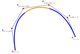
In the mathematical subfield of numerical analysis, a B-spline or basis spline is a spline function that has minimal support with respect to a given degree, smoothness, and domain partition. Any spline function of given degree can be expressed as a linear combination of B-splines of that degree. Cardinal B-splines have knots that are equidistant from each other. B-splines can be used for curve-fitting and numerical differentiation of experimental data.

In the mathematical field of numerical analysis, Runge's phenomenon is a problem of oscillation at the edges of an interval that occurs when using polynomial interpolation with polynomials of high degree over a set of equispaced interpolation points. It was discovered by Carl David Tolmé Runge (1901) when exploring the behavior of errors when using polynomial interpolation to approximate certain functions. The discovery was important because it shows that going to higher degrees does not always improve accuracy. The phenomenon is similar to the Gibbs phenomenon in Fourier series approximations.
In numerical analysis, polynomial interpolation is the interpolation of a given data set by the polynomial of lowest possible degree that passes through the points of the dataset.
In the mathematical field of numerical analysis, a Newton polynomial, named after its inventor Isaac Newton, is an interpolation polynomial for a given set of data points. The Newton polynomial is sometimes called Newton's divided differences interpolation polynomial because the coefficients of the polynomial are calculated using Newton's divided differences method.
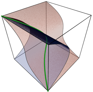
Algebraic varieties are the central objects of study in algebraic geometry, a sub-field of mathematics. Classically, an algebraic variety is defined as the set of solutions of a system of polynomial equations over the real or complex numbers. Modern definitions generalize this concept in several different ways, while attempting to preserve the geometric intuition behind the original definition.

In algebraic geometry, an affine variety, or affine algebraic variety, over an algebraically closed field k is the zero-locus in the affine space kn of some finite family of polynomials of n variables with coefficients in k that generate a prime ideal. If the condition of generating a prime ideal is removed, such a set is called an (affine) algebraic set. A Zariski open subvariety of an affine variety is called a quasi-affine variety.
In mathematics, a spline is a special function defined piecewise by polynomials. In interpolating problems, spline interpolation is often preferred to polynomial interpolation because it yields similar results, even when using low degree polynomials, while avoiding Runge's phenomenon for higher degrees.
In the mathematical field of numerical analysis, spline interpolation is a form of interpolation where the interpolant is a special type of piecewise polynomial called a spline. That is, instead of fitting a single, high-degree polynomial to all of the values at once, spline interpolation fits low-degree polynomials to small subsets of the values, for example, fitting nine cubic polynomials between each of the pairs of ten points, instead of fitting a single degree-ten polynomial to all of them. Spline interpolation is often preferred over polynomial interpolation because the interpolation error can be made small even when using low-degree polynomials for the spline. Spline interpolation also avoids the problem of Runge's phenomenon, in which oscillation can occur between points when interpolating using high-degree polynomials.
In numerical analysis, a cubic Hermite spline or cubic Hermite interpolator is a spline where each piece is a third-degree polynomial specified in Hermite form, that is, by its values and first derivatives at the end points of the corresponding domain interval.
In mathematics, trigonometric interpolation is interpolation with trigonometric polynomials. Interpolation is the process of finding a function which goes through some given data points. For trigonometric interpolation, this function has to be a trigonometric polynomial, that is, a sum of sines and cosines of given periods. This form is especially suited for interpolation of periodic functions.
In mathematics, the Lebesgue constants (depending on a set of nodes and of its size) give an idea of how good the interpolant of a function (at the given nodes) is in comparison with the best polynomial approximation of the function (the degree of the polynomials are fixed). The Lebesgue constant for polynomials of degree at most n and for the set of n + 1 nodes T is generally denoted by Λn(T ). These constants are named after Henri Lebesgue.
In applied mathematics, polyharmonic splines are used for function approximation and data interpolation. They are very useful for interpolating and fitting scattered data in many dimensions. Special cases include thin plate splines and natural cubic splines in one dimension.
In the mathematical field of numerical analysis, monotone cubic interpolation is a variant of cubic interpolation that preserves monotonicity of the data set being interpolated.
In numerical analysis, multivariate interpolation is interpolation on functions of more than one variable; when the variates are spatial coordinates, it is also known as spatial interpolation.

The finite element method (FEM) is a popular method for numerically solving differential equations arising in engineering and mathematical modeling. Typical problem areas of interest include the traditional fields of structural analysis, heat transfer, fluid flow, mass transport, and electromagnetic potential.
Smoothing splines are function estimates, , obtained from a set of noisy observations of the target , in order to balance a measure of goodness of fit of to with a derivative based measure of the smoothness of . They provide a means for smoothing noisy data. The most familiar example is the cubic smoothing spline, but there are many other possibilities, including for the case where is a vector quantity.
In mathematics, discrete Chebyshev polynomials, or Gram polynomials, are a type of discrete orthogonal polynomials used in approximation theory, introduced by Pafnuty Chebyshev and rediscovered by Gram. They were later found to be applicable to various algebraic properties of spin angular momentum.
In the mathematical fields of numerical analysis and approximation theory, box splines are piecewise polynomial functions of several variables. Box splines are considered as a multivariate generalization of basis splines (B-splines) and are generally used for multivariate approximation/interpolation. Geometrically, a box spline is the shadow (X-ray) of a hypercube projected down to a lower-dimensional space. Box splines and simplex splines are well studied special cases of polyhedral splines which are defined as shadows of general polytopes.


