There are several kinds of mean in mathematics, especially in statistics. Each mean serves to summarize a given group of data, often to better understand the overall value of a given data set.
Numerical analysis is the study of algorithms that use numerical approximation for the problems of mathematical analysis. It is the study of numerical methods that attempt at finding approximate solutions of problems rather than the exact ones. Numerical analysis finds application in all fields of engineering and the physical sciences, and in the 21st century also the life and social sciences, medicine, business and even the arts. Current growth in computing power has enabled the use of more complex numerical analysis, providing detailed and realistic mathematical models in science and engineering. Examples of numerical analysis include: ordinary differential equations as found in celestial mechanics, numerical linear algebra in data analysis, and stochastic differential equations and Markov chains for simulating living cells in medicine and biology.
A finite difference is a mathematical expression of the form f (x + b) − f (x + a). If a finite difference is divided by b − a, one gets a difference quotient. The approximation of derivatives by finite differences plays a central role in finite difference methods for the numerical solution of differential equations, especially boundary value problems.

In signal processing, a digital filter is a system that performs mathematical operations on a sampled, discrete-time signal to reduce or enhance certain aspects of that signal. This is in contrast to the other major type of electronic filter, the analog filter, which is typically an electronic circuit operating on continuous-time analog signals.

In analysis, numerical integration comprises a broad family of algorithms for calculating the numerical value of a definite integral, and by extension, the term is also sometimes used to describe the numerical solution of differential equations. This article focuses on calculation of definite integrals.
A numerically controlled oscillator (NCO) is a digital signal generator which creates a synchronous, discrete-time, discrete-valued representation of a waveform, usually sinusoidal. NCOs are often used in conjunction with a digital-to-analog converter (DAC) at the output to create a direct digital synthesizer (DDS).

Numerical methods for ordinary differential equations are methods used to find numerical approximations to the solutions of ordinary differential equations (ODEs). Their use is also known as "numerical integration", although this term can also refer to the computation of integrals.

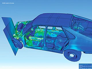
Computational fluid dynamics (CFD) is a branch of fluid mechanics that uses numerical analysis and data structures to analyze and solve problems that involve fluid flows. Computers are used to perform the calculations required to simulate the free-stream flow of the fluid, and the interaction of the fluid with surfaces defined by boundary conditions. With high-speed supercomputers, better solutions can be achieved, and are often required to solve the largest and most complex problems. Ongoing research yields software that improves the accuracy and speed of complex simulation scenarios such as transonic or turbulent flows. Initial validation of such software is typically performed using experimental apparatus such as wind tunnels. In addition, previously performed analytical or empirical analysis of a particular problem can be used for comparison. A final validation is often performed using full-scale testing, such as flight tests.
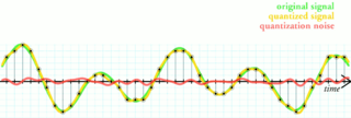
Quantization, in mathematics and digital signal processing, is the process of mapping input values from a large set to output values in a (countable) smaller set, often with a finite number of elements. Rounding and truncation are typical examples of quantization processes. Quantization is involved to some degree in nearly all digital signal processing, as the process of representing a signal in digital form ordinarily involves rounding. Quantization also forms the core of essentially all lossy compression algorithms.
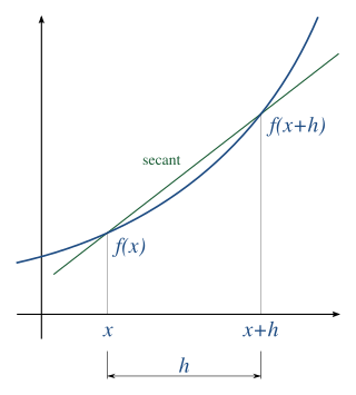
In numerical analysis, numerical differentiation algorithms estimate the derivative of a mathematical function or function subroutine using values of the function and perhaps other knowledge about the function.
In mathematics, the discrete Laplace operator is an analog of the continuous Laplace operator, defined so that it has meaning on a graph or a discrete grid. For the case of a finite-dimensional graph, the discrete Laplace operator is more commonly called the Laplacian matrix.
Numerical methods for partial differential equations is the branch of numerical analysis that studies the numerical solution of partial differential equations (PDEs).

Computational electromagnetics (CEM), computational electrodynamics or electromagnetic modeling is the process of modeling the interaction of electromagnetic fields with physical objects and the environment.
Flux limiters are used in high resolution schemes – numerical schemes used to solve problems in science and engineering, particularly fluid dynamics, described by partial differential equations (PDEs). They are used in high resolution schemes, such as the MUSCL scheme, to avoid the spurious oscillations (wiggles) that would otherwise occur with high order spatial discretization schemes due to shocks, discontinuities or sharp changes in the solution domain. Use of flux limiters, together with an appropriate high resolution scheme, make the solutions total variation diminishing (TVD).
In numerical analysis, finite-difference methods (FDM) are a class of numerical techniques for solving differential equations by approximating derivatives with finite differences. Both the spatial domain and time interval are discretized, or broken into a finite number of steps, and the value of the solution at these discrete points is approximated by solving algebraic equations containing finite differences and values from nearby points.
In applied mathematics, the numerical sign problem is the problem of numerically evaluating the integral of a highly oscillatory function of a large number of variables. Numerical methods fail because of the near-cancellation of the positive and negative contributions to the integral. Each has to be integrated to very high precision in order for their difference to be obtained with useful accuracy.
The finite element method (FEM) is a popular method for numerically solving differential equations arising in engineering and mathematical modeling. Typical problem areas of interest include the traditional fields of structural analysis, heat transfer, fluid flow, mass transport, and electromagnetic potential.
A multidimensional signal is a function of M independent variables where . Real world signals, which are generally continuous time signals, have to be discretized (sampled) in order to ensure that digital systems can be used to process the signals. It is during this process of discretization where sampling comes into picture. Although there are many ways of obtaining a discrete representation of a continuous time signal, periodic sampling is by far the simplest scheme. Theoretically, sampling can be performed with respect to any set of points. But practically, sampling is carried out with respect to a set of points that have a certain algebraic structure. Such structures are called lattices. Mathematically, the process of sampling an -dimensional signal can be written as:
Fluid motion is governed by the Navier–Stokes equations, a set of coupled and nonlinear partial differential equations derived from the basic laws of conservation of mass, momentum and energy. The unknowns are usually the flow velocity, the pressure and density and temperature. The analytical solution of this equation is impossible hence scientists resort to laboratory experiments in such situations. The answers delivered are, however, usually qualitatively different since dynamical and geometric similitude are difficult to enforce simultaneously between the lab experiment and the prototype. Furthermore, the design and construction of these experiments can be difficult, particularly for stratified rotating flows. Computational fluid dynamics (CFD) is an additional tool in the arsenal of scientists. In its early days CFD was often controversial, as it involved additional approximation to the governing equations and raised additional (legitimate) issues. Nowadays CFD is an established discipline alongside theoretical and experimental methods. This position is in large part due to the exponential growth of computer power which has allowed us to tackle ever larger and more complex problems.


