In quantum mechanics, bra–ket notation, or Dirac notation, is ubiquitous. The notation uses the angle brackets, "" and "", and a vertical bar "", to construct "bras" and "kets".

The wave equation is an important second-order linear partial differential equation for the description of waves—as they occur in classical physics—such as mechanical waves or light waves. It arises in fields like acoustics, electromagnetics, and fluid dynamics.

In mathematics and physics, Laplace's equation is a second-order partial differential equation named after Pierre-Simon Laplace who first studied its properties. This is often written as

In particle physics, the Dirac equation is a relativistic wave equation derived by British physicist Paul Dirac in 1928. In its free form, or including electromagnetic interactions, it describes all spin-½ massive particles such as electrons and quarks for which parity is a symmetry. It is consistent with both the principles of quantum mechanics and the theory of special relativity, and was the first theory to account fully for special relativity in the context of quantum mechanics. It was validated by accounting for the fine details of the hydrogen spectrum in a completely rigorous way.
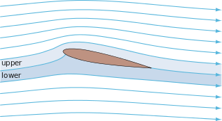
In fluid dynamics, potential flow describes the velocity field as the gradient of a scalar function: the velocity potential. As a result, a potential flow is characterized by an irrotational velocity field, which is a valid approximation for several applications. The irrotationality of a potential flow is due to the curl of the gradient of a scalar always being equal to zero.
A wave function in quantum physics is a mathematical description of the quantum state of an isolated quantum system. The wave function is a complex-valued probability amplitude, and the probabilities for the possible results of measurements made on the system can be derived from it. The most common symbols for a wave function are the Greek letters ψ and Ψ.
In physics, charge conjugation is a transformation that switches all particles with their corresponding antiparticles, thus changing the sign of all charges: not only electric charge but also the charges relevant to other forces. The term C-symmetry is an abbreviation of the phrase "charge conjugation symmetry", and is used in discussions of the symmetry of physical laws under charge-conjugation. Other important discrete symmetries are P-symmetry (parity) and T-symmetry.
In mechanics and geometry, the 3D rotation group, often denoted SO(3), is the group of all rotations about the origin of three-dimensional Euclidean space under the operation of composition. By definition, a rotation about the origin is a transformation that preserves the origin, Euclidean distance, and orientation. Every non-trivial rotation is determined by its axis of rotation and its angle of rotation. Composing two rotations results in another rotation; every rotation has a unique inverse rotation; and the identity map satisfies the definition of a rotation. Owing to the above properties, the set of all rotations is a group under composition. Rotations are not commutative, making it a nonabelian group. Moreover, the rotation group has a natural structure as a manifold for which the group operations are smoothly differentiable; so it is in fact a Lie group. It is compact and has dimension 3.
In mathematics, a self-adjoint operator on a finite-dimensional complex vector space V with inner product is a linear map A that is its own adjoint: for all vectors v and w. If V is finite-dimensional with a given orthonormal basis, this is equivalent to the condition that the matrix of A is a Hermitian matrix, i.e., equal to its conjugate transpose A∗. By the finite-dimensional spectral theorem, V has an orthonormal basis such that the matrix of A relative to this basis is a diagonal matrix with entries in the real numbers. In this article, we consider generalizations of this concept to operators on Hilbert spaces of arbitrary dimension.
In physics, an operator is a function over a space of physical states onto another space of physical states. The simplest example of the utility of operators is the study of symmetry. Because of this, they are very useful tools in classical mechanics. Operators are even more important in quantum mechanics, where they form an intrinsic part of the formulation of the theory.
In physics, the S-matrix or scattering matrix relates the initial state and the final state of a physical system undergoing a scattering process. It is used in quantum mechanics, scattering theory and quantum field theory (QFT).
In physics, the Hamilton–Jacobi equation, named after William Rowan Hamilton and Carl Gustav Jacob Jacobi, is an alternative formulation of classical mechanics, equivalent to other formulations such as Newton's laws of motion, Lagrangian mechanics and Hamiltonian mechanics. The Hamilton–Jacobi equation is particularly useful in identifying conserved quantities for mechanical systems, which may be possible even when the mechanical problem itself cannot be solved completely.

In mathematics, an ordered basis of a vector space of finite dimension n allows representing uniquely any element of the vector space by a coordinate vector, which is a sequence of n scalars called coordinates. If two different bases are considered, the coordinate vector that represents a vector v on one basis is, in general, different from the coordinate vector that represents v on the other basis. A change of basis consists of converting every assertion expressed in terms of coordinates relative to one basis into an assertion expressed in terms of coordinates relative to the other basis.

In theoretical physics, the (one-dimensional) nonlinear Schrödinger equation (NLSE) is a nonlinear variation of the Schrödinger equation. It is a classical field equation whose principal applications are to the propagation of light in nonlinear optical fibers and planar waveguides and to Bose–Einstein condensates confined to highly anisotropic cigar-shaped traps, in the mean-field regime. Additionally, the equation appears in the studies of small-amplitude gravity waves on the surface of deep inviscid (zero-viscosity) water; the Langmuir waves in hot plasmas; the propagation of plane-diffracted wave beams in the focusing regions of the ionosphere; the propagation of Davydov's alpha-helix solitons, which are responsible for energy transport along molecular chains; and many others. More generally, the NLSE appears as one of universal equations that describe the evolution of slowly varying packets of quasi-monochromatic waves in weakly nonlinear media that have dispersion. Unlike the linear Schrödinger equation, the NLSE never describes the time evolution of a quantum state. The 1D NLSE is an example of an integrable model.
In mathematical analysis an oscillatory integral is a type of distribution. Oscillatory integrals make rigorous many arguments that, on a naive level, appear to use divergent integrals. It is possible to represent approximate solution operators for many differential equations as oscillatory integrals.
In mathematics, the Prolate spheroidal wave functions (PSWF) are a set of orthogonal bandlimited functions. They are eigenfunctions of a timelimiting operation followed by a lowpassing operation. Let denote the time truncation operator, such that if and only if is timelimited within . Similarly, let denote an ideal low-pass filtering operator, such that if and only if is bandlimited within ;\Omega ]} . The operator turns out to be linear, bounded and self-adjoint. For we denote with the n-th eigenfunction, defined as
In mathematics, Liouville's formula, also known as the Abel-Jacobi-Liouville Identity, is an equation that expresses the determinant of a square-matrix solution of a first-order system of homogeneous linear differential equations in terms of the sum of the diagonal coefficients of the system. The formula is named after the French mathematician Joseph Liouville. Jacobi's formula provides another representation of the same mathematical relationship.
In mathematics, the spectral theory of ordinary differential equations is the part of spectral theory concerned with the determination of the spectrum and eigenfunction expansion associated with a linear ordinary differential equation. In his dissertation Hermann Weyl generalized the classical Sturm–Liouville theory on a finite closed interval to second order differential operators with singularities at the endpoints of the interval, possibly semi-infinite or infinite. Unlike the classical case, the spectrum may no longer consist of just a countable set of eigenvalues, but may also contain a continuous part. In this case the eigenfunction expansion involves an integral over the continuous part with respect to a spectral measure, given by the Titchmarsh–Kodaira formula. The theory was put in its final simplified form for singular differential equations of even degree by Kodaira and others, using von Neumann's spectral theorem. It has had important applications in quantum mechanics, operator theory and harmonic analysis on semisimple Lie groups.
Symmetries in quantum mechanics describe features of spacetime and particles which are unchanged under some transformation, in the context of quantum mechanics, relativistic quantum mechanics and quantum field theory, and with applications in the mathematical formulation of the standard model and condensed matter physics. In general, symmetry in physics, invariance, and conservation laws, are fundamentally important constraints for formulating physical theories and models. In practice, they are powerful methods for solving problems and predicting what can happen. While conservation laws do not always give the answer to the problem directly, they form the correct constraints and the first steps to solving a multitude of problems.
The Schamel equation (S-equation) is a nonlinear partial differential equation of first order in time and third order in space. Similar to a Korteweg de Vries equation (KdV), it describes the development of a localized, coherent wave structure that propagates in a nonlinear dispersive medium. It was first derived in 1973 by Hans Schamel to describe the effects of electron trapping in the trough of the potential of a solitary electrostatic wave structure travelling with ion acoustic speed in a two-component plasma. It now applies to various localized pulse dynamics such as:


