
The Antarctic Circumpolar Current (ACC) is an ocean current that flows clockwise from west to east around Antarctica. An alternative name for the ACC is the West Wind Drift. The ACC is the dominant circulation feature of the Southern Ocean and has a mean transport estimated at 100–150 Sverdrups, or possibly even higher, making it the largest ocean current. The current is circumpolar due to the lack of any landmass connecting with Antarctica and this keeps warm ocean waters away from Antarctica, enabling that continent to maintain its huge ice sheet.
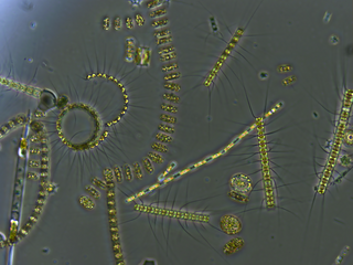
Phytoplankton are the autotrophic (self-feeding) components of the plankton community and a key part of ocean and freshwater ecosystems. The name comes from the Greek words φυτόν, meaning 'plant', and πλαγκτός, meaning 'wanderer' or 'drifter'.
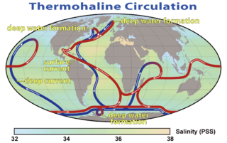
Thermohaline circulation (THC) is a part of the large-scale ocean circulation that is driven by global density gradients created by surface heat and freshwater fluxes. The adjective thermohaline derives from thermo- referring to temperature and -haline referring to salt content, factors which together determine the density of sea water. Wind-driven surface currents travel polewards from the equatorial Atlantic Ocean, cooling en route, and eventually sinking at high latitudes. This dense water then flows into the ocean basins. While the bulk of it upwells in the Southern Ocean, the oldest waters upwell in the North Pacific. Extensive mixing therefore takes place between the ocean basins, reducing differences between them and making the Earth's oceans a global system. The water in these circuits transport both energy and mass around the globe. As such, the state of the circulation has a large impact on the climate of the Earth.
Isotopic labeling is a technique used to track the passage of an isotope through a reaction, metabolic pathway, or cell. The reactant is 'labeled' by replacing specific atoms by their isotope. The reactant is then allowed to undergo the reaction. The position of the isotopes in the products is measured to determine the sequence the isotopic atom followed in the reaction or the cell's metabolic pathway. The nuclides used in isotopic labeling may be stable nuclides or radionuclides. In the latter case, the labeling is called radiolabeling.
A pycnocline is the cline or layer where the density gradient is greatest within a body of water. An ocean current is generated by the forces such as breaking waves, temperature and salinity differences, wind, Coriolis effect, and tides caused by the gravitational pull of celestial bodies. In addition, the physical properties in a pycnocline driven by density gradients also affect the flows and vertical profiles in the ocean. These changes can be connected to the transport of heat, salt, and nutrients through the ocean, and the pycnocline diffusion controls upwelling.
High-nutrient, low-chlorophyll (HNLC) regions are regions of the ocean where the abundance of phytoplankton is low and fairly constant despite the availability of macronutrients. Phytoplankton rely on a suite of nutrients for cellular function. Macronutrients are generally available in higher quantities in surface ocean waters, and are the typical components of common garden fertilizers. Micronutrients are generally available in lower quantities and include trace metals. Macronutrients are typically available in millimolar concentrations, while micronutrients are generally available in micro- to nanomolar concentrations. In general, nitrogen tends to be a limiting ocean nutrient, but in HNLC regions it is never significantly depleted. Instead, these regions tend to be limited by low concentrations of metabolizable iron. Iron is a critical phytoplankton micronutrient necessary for enzyme catalysis and electron transport.
In biological oceanography, critical depth is defined as a hypothetical surface mixing depth where phytoplankton growth is precisely matched by losses of phytoplankton biomass within the depth interval. This concept is useful for understanding the initiation of phytoplankton blooms.
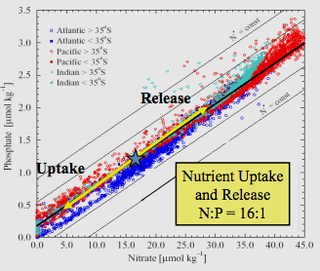
The Redfield ratio or Redfield stoichiometry is the consistent atomic ratio of carbon, nitrogen and phosphorus found in marine phytoplankton and throughout the deep oceans.
The environmental isotopes are a subset of isotopes, both stable and radioactive, which are the object of isotope geochemistry. They are primarily used as tracers to see how things move around within the ocean-atmosphere system, within terrestrial biomes, within the Earth's surface, and between these broad domains.
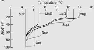
The oceanic or limnological mixed layer is a layer in which active turbulence has homogenized some range of depths. The surface mixed layer is a layer where this turbulence is generated by winds, surface heat fluxes, or processes such as evaporation or sea ice formation which result in an increase in salinity. The atmospheric mixed layer is a zone having nearly constant potential temperature and specific humidity with height. The depth of the atmospheric mixed layer is known as the mixing height. Turbulence typically plays a role in the formation of fluid mixed layers.

Ocean fertilization or ocean nourishment is a type of technology for carbon dioxide removal from the ocean based on the purposeful introduction of plant nutrients to the upper ocean to increase marine food production and to remove carbon dioxide from the atmosphere. Ocean nutrient fertilization, for example iron fertilization, could stimulate photosynthesis in phytoplankton. The phytoplankton would convert the ocean's dissolved carbon dioxide into carbohydrate, some of which would sink into the deeper ocean before oxidizing. More than a dozen open-sea experiments confirmed that adding iron to the ocean increases photosynthesis in phytoplankton by up to 30 times.

Thin layers are concentrated aggregations of phytoplankton and zooplankton in coastal and offshore waters that are vertically compressed to thicknesses ranging from several centimeters up to a few meters and are horizontally extensive, sometimes for kilometers. Generally, thin layers have three basic criteria: 1) they must be horizontally and temporally persistent; 2) they must not exceed a critical threshold of vertical thickness; and 3) they must exceed a critical threshold of maximum concentration. The precise values for critical thresholds of thin layers has been debated for a long time due to the vast diversity of plankton, instrumentation, and environmental conditions. Thin layers have distinct biological, chemical, optical, and acoustical signatures which are difficult to measure with traditional sampling techniques such as nets and bottles. However, there has been a surge in studies of thin layers within the past two decades due to major advances in technology and instrumentation. Phytoplankton are often measured by optical instruments that can detect fluorescence such as LIDAR, and zooplankton are often measured by acoustic instruments that can detect acoustic backscattering such as ABS. These extraordinary concentrations of plankton have important implications for many aspects of marine ecology, as well as for ocean optics and acoustics. Zooplankton thin layers are often found slightly under phytoplankton layers because many feed on them. Thin layers occur in a wide variety of ocean environments, including estuaries, coastal shelves, fjords, bays, and the open ocean, and they are often associated with some form of vertical structure in the water column, such as pycnoclines, and in zones of reduced flow.

In physical oceanography, Langmuir circulation consists of a series of shallow, slow, counter-rotating vortices at the ocean's surface aligned with the wind. These circulations are developed when wind blows steadily over the sea surface. Irving Langmuir discovered this phenomenon after observing windrows of seaweed in the Sargasso Sea in 1927. Langmuir circulations circulate within the mixed layer; however, it is not yet so clear how strongly they can cause mixing at the base of the mixed layer.
The deep chlorophyll maximum (DCM), also called the subsurface chlorophyll maximum, is the region below the surface of water with the maximum concentration of chlorophyll. The DCM generally exists at the same depth as the nutricline, the region of the ocean where the greatest change in the nutrient concentration occurs with depth.

The North Pacific Subtropical Gyre (NPSG) is the largest contiguous ecosystem on earth. In oceanography, a subtropical gyre is a ring-like system of ocean currents rotating clockwise in the Northern Hemisphere and counterclockwise in the Southern Hemisphere caused by the Coriolis Effect. They generally form in large open ocean areas that lie between land masses.
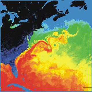
Cold core rings are a type of oceanic eddy, which are characterized as unstable, time-dependent swirling, independent ‘cells’ that separate from their respective ocean current and move into water bodies with different physical, chemical, and biological characteristics, often bringing the physical, chemical, and biological characteristics of the waters of their origin into the water bodies into which they travel. Their size can range from 1 millimeter (0.039 in) to over 10,000 kilometers (6,200 mi) in diameter with depths over 5 kilometers (3.1 mi). Cold core rings are the product of warm water currents wrapping around a colder water mass as it deviates away from its respective current. The direction an eddy swirls can be categorized as either cyclonic or anticyclonic, which is, in the Northern Hemisphere, counterclockwise and clockwise respectively, and in the Southern Hemisphere, clockwise and counterclockwise respectively as a result of the Coriolis effect. Although eddies have large amounts of kinetic energy, their rotation is relatively quick to decrease in relation to the amount of viscous friction in water. They typically last for a few weeks to a year. The nature of eddies are such that the center of the eddy, the outer swirling ring, and the surrounding waters are well stratified and maintain all of their distinctive physical, chemical, and biological properties throughout the eddy’s lifetime, before losing their distinctive characteristics at the end of the life of the cold core ring.
The residence time of a fluid parcel is the total time that the parcel has spent inside a control volume (e.g.: a chemical reactor, a lake, a human body). The residence time of a set of parcels is quantified in terms of the frequency distribution of the residence time in the set, which is known as residence time distribution (RTD), or in terms of its average, known as mean residence time.
Nutrient cycling in the Columbia River Basin involves the transport of nutrients through the system, as well as transformations from among dissolved, solid, and gaseous phases, depending on the element. The elements that constitute important nutrient cycles include macronutrients such as nitrogen, silicate, phosphorus, and micronutrients, which are found in trace amounts, such as iron. Their cycling within a system is controlled by many biological, chemical, and physical processes.

The viral shunt is a mechanism that prevents marine microbial particulate organic matter (POM) from migrating up trophic levels by recycling them into dissolved organic matter (DOM), which can be readily taken up by microorganisms. The DOM recycled by the viral shunt pathway is comparable to the amount generated by the other main sources of marine DOM.
Low-nutrient, low-chlorophyll (LNLC)regions are aquatic zones that are low in nutrients and consequently have low rate of primary production, as indicated by low chlorophyll concentrations. These regions can be described as oligotrophic, and about 75% of the world's oceans encompass LNLC regions. A majority of LNLC regions are associated with subtropical gyres but are also present in areas of the Mediterranean Sea, and some inland lakes. Physical processes limit nutrient availability in LNLC regions, which favors nutrient recycling in the photic zone and selects for smaller phytoplankton species. LNLC regions are generally not found near coasts, owing to the fact that coastal areas receive more nutrients from terrestrial sources and upwelling. In marine systems, seasonal and decadal variability of primary productivity in LNLC regions is driven in part by large-scale climatic regimes leading to important effects on the global carbon cycle and the oceanic carbon cycle.

