Incidence structure

Last updated
Examples of incidence structures:
Example 1: points and lines of the Euclidean plane (top)
Example 2: points and circles (middle),
Example 3: finite incidence structure defined by an incidence matrix (bottom) Inzidenz-struktur.svg
Examples of incidence structures:
Example 1: points and lines of the Euclidean plane (top)
Example 2: points and circles (middle),
Example 3: finite incidence structure defined by an incidence matrix (bottom)

In mathematics, an incidence structure is an abstract system consisting of two types of objects and a single relationship between these types of objects. Consider the points and lines of the Euclidean plane as the two types of objects and ignore all the properties of this geometry except for the relation of which points are on which lines for all points and lines. What is left is the incidence structure of the Euclidean plane.

Contents

Incidence structures are most often considered in the geometrical context where they are abstracted from, and hence generalize, planes (such as affine, projective, and Möbius planes), but the concept is very broad and not limited to geometric settings. Even in a geometric setting, incidence structures are not limited to just points and lines; higher-dimensional objects (planes, solids, n-spaces, conics, etc.) can be used. The study of finite structures is sometimes called finite geometry. [1]

Formal definition and terminology

An incidence structure is a triple (P, L, I) where P is a set whose elements are called points, L is a distinct set whose elements are called lines and IP × L is the incidence relation. The elements of I are called flags. If (p, l) is in I then one may say that point p "lies on" line l or that the line l "passes through" point p. A more "symmetric" terminology, to reflect the symmetric nature of this relation, is that "p is incident with l" or that "l is incident with p" and uses the notation p I l synonymously with (p, l) ∈ I. [2]

In some common situations L may be a set of subsets of P in which case incidence I will be containment (p I l if and only if p is a member of l). Incidence structures of this type are called set-theoretic. [3] This is not always the case, for example, if P is a set of vectors and L a set of square matrices, we may define

This example also shows that while the geometric language of points and lines is used, the object types need not be these geometric objects.

Examples

An incidence structure is uniform if each line is incident with the same number of points. Each of these examples, except the second, is uniform with three points per line.

Graphs

Any graph (which need not be simple; loops and multiple edges are allowed) is a uniform incidence structure with two points per line. For these examples, the vertices of the graph form the point set, the edges of the graph form the line set, and incidence means that a vertex is an endpoint of an edge.

Linear spaces

Incidence structures are seldom studied in their full generality; it is typical to study incidence structures that satisfy some additional axioms. For instance, a partial linear space is an incidence structure that satisfies:

  1. Any two distinct points are incident with at most one common line, and
  2. Every line is incident with at least two points.

If the first axiom above is replaced by the stronger:

  1. Any two distinct points are incident with exactly one common line,

the incidence structure is called a linear space . [4] [5]

Nets

A more specialized example is a k-net. This is an incidence structure in which the lines fall into kparallel classes, so that two lines in the same parallel class have no common points, but two lines in different classes have exactly one common point, and each point belongs to exactly one line from each parallel class. An example of a k-net is the set of points of an affine plane together with k parallel classes of affine lines.

Dual structure

If we interchange the role of "points" and "lines" in

we obtain the dual structure,

where I is the converse relation of I. It follows immediately from the definition that:

This is an abstract version of projective duality. [2]

A structure C that is isomorphic to its dual C is called self-dual. The Fano plane above is a self-dual incidence structure.

Other terminology

The concept of an incidence structure is very simple and has arisen in several disciplines, each introducing its own vocabulary and specifying the types of questions that are typically asked about these structures. Incidence structures use a geometric terminology, but in graph theoretic terms they are called hypergraphs and in design theoretic terms they are called block designs. They are also known as a set system or family of sets in a general context.

Hypergraphs

Seven points are elements of seven lines in the Fano plane Fano plane with nimber labels.svg
Seven points are elements of seven lines in the Fano plane

Each hypergraph or set system can be regarded as an incidence structure in which the universal set plays the role of "points", the corresponding family of sets plays the role of "lines" and the incidence relation is set membership "". Conversely, every incidence structure can be viewed as a hypergraph by identifying the lines with the sets of points that are incident with them.

Block designs

A (general) block design is a set X together with a family F of subsets of X (repeated subsets are allowed). Normally a block design is required to satisfy numerical regularity conditions. As an incidence structure, X is the set of points and F is the set of lines, usually called blocks in this context (repeated blocks must have distinct names, so F is actually a set and not a multiset). If all the subsets in F have the same size, the block design is called uniform. If each element of X appears in the same number of subsets, the block design is said to be regular. The dual of a uniform design is a regular design and vice versa.

Example: Fano plane

Consider the block design/hypergraph given by:

This incidence structure is called the Fano plane. As a block design it is both uniform and regular.

In the labeling given, the lines are precisely the subsets of the points that consist of three points whose labels add up to zero using nim addition. Alternatively, each number, when written in binary, can be identified with a non-zero vector of length three over the binary field. Three vectors that generate a subspace form a line; in this case, that is equivalent to their vector sum being the zero vector.

Representations

Incidence structures may be represented in many ways. If the sets P and L are finite these representations can compactly encode all the relevant information concerning the structure.

Incidence matrix

The incidence matrix of a (finite) incidence structure is a (0,1) matrix that has its rows indexed by the points {pi} and columns indexed by the lines {lj} where the ij-th entry is a 1 if pi I lj and 0 otherwise. [lower-alpha 1] An incidence matrix is not uniquely determined since it depends upon the arbitrary ordering of the points and the lines. [6]

The non-uniform incidence structure pictured above (example number 2) is given by:

An incidence matrix for this structure is:

which corresponds to the incidence table:

Ilmnopq
A000110
B000011
C100000
D001000
E100000
P111101

If an incidence structure C has an incidence matrix M, then the dual structure C has the transpose matrix MT as its incidence matrix (and is defined by that matrix).

An incidence structure is self-dual if there exists an ordering of the points and lines so that the incidence matrix constructed with that ordering is a symmetric matrix.

With the labels as given in example number 1 above and with points ordered A, B, C, D, G, F, E and lines ordered l, p, n, s, r, m, q, the Fano plane has the incidence matrix:

Since this is a symmetric matrix, the Fano plane is a self-dual incidence structure.

Pictorial representations

An incidence figure (that is, a depiction of an incidence structure), is constructed by representing the points by dots in a plane and having some visual means of joining the dots to correspond to lines. [6] The dots may be placed in any manner, there are no restrictions on distances between points or any relationships between points. In an incidence structure there is no concept of a point being between two other points; the order of points on a line is undefined. Compare this with ordered geometry, which does have a notion of betweenness. The same statements can be made about the depictions of the lines. In particular, lines need not be depicted by "straight line segments" (see examples 1, 3 and 4 above). As with the pictorial representation of graphs, the crossing of two "lines" at any place other than a dot has no meaning in terms of the incidence structure; it is only an accident of the representation. These incidence figures may at times resemble graphs, but they aren't graphs unless the incidence structure is a graph.

Realizability

Incidence structures can be modelled by points and curves in the Euclidean plane with the usual geometric meaning of incidence. Some incidence structures admit representation by points and (straight) lines. Structures that can be are called realizable. If no ambient space is mentioned then the Euclidean plane is assumed. The Fano plane (example 1 above) is not realizable since it needs at least one curve. The Möbius–Kantor configuration (example 4 above) is not realizable in the Euclidean plane, but it is realizable in the complex plane. [7] On the other hand, examples 2 and 5 above are realizable and the incidence figures given there demonstrate this. Steinitz (1894) [8] has shown that n3-configurations (incidence structures with n points and n lines, three points per line and three lines through each point) are either realizable or require the use of only one curved line in their representations. [9] The Fano plane is the unique (73) and the Möbius–Kantor configuration is the unique (83).

Incidence graph (Levi graph)

Heawood graph with labeling Fano plane-Levi graph.svg
Heawood graph with labeling

Each incidence structure C corresponds to a bipartite graph called the Levi graph or incidence graph of the structure. As any bipartite graph is two-colorable, the Levi graph can be given a black and white vertex coloring, where black vertices correspond to points and white vertices correspond to lines of C. The edges of this graph correspond to the flags (incident point/line pairs) of the incidence structure. The original Levi graph was the incidence graph of the generalized quadrangle of order two (example 3 above), [10] but the term has been extended by H.S.M. Coxeter [11] to refer to an incidence graph of any incidence structure. [12]

Levi graph of the Mobius-Kantor configuration (#4) Mobius-Kantor unit distance.svg
Levi graph of the Möbius–Kantor configuration (#4)

Levi graph examples

The Levi graph of the Fano plane is the Heawood graph. Since the Heawood graph is connected and vertex-transitive, there exists an automorphism (such as the one defined by a reflection about the vertical axis in the figure of the Heawood graph) interchanging black and white vertices. This, in turn, implies that the Fano plane is self-dual.

The specific representation, on the left, of the Levi graph of the Möbius–Kantor configuration (example 4 above) illustrates that a rotation of π/4 about the center (either clockwise or counterclockwise) of the diagram interchanges the blue and red vertices and maps edges to edges. That is to say that there exists a color interchanging automorphism of this graph. Consequently, the incidence structure known as the Möbius–Kantor configuration is self-dual.

Generalization

It is possible to generalize the notion of an incidence structure to include more than two types of objects. A structure with k types of objects is called an incidence structure of rankk or a rankkgeometry. [12] Formally these are defined as k + 1 tuples S = (P1, P2, ..., Pk, I) with PiPj = ∅ and

The Levi graph for these structures is defined as a multipartite graph with vertices corresponding to each type being colored the same.

See also

Notes

  1. The other convention of indexing the rows by lines and the columns by points is also widely used.

Related Research Articles

<span class="mw-page-title-main">Dual polyhedron</span> Polyhedron associated with another by swapping vertices for faces

In geometry, every polyhedron is associated with a second dual structure, where the vertices of one correspond to the faces of the other, and the edges between pairs of vertices of one correspond to the edges between pairs of faces of the other. Such dual figures remain combinatorial or abstract polyhedra, but not all can also be constructed as geometric polyhedra. Starting with any given polyhedron, the dual of its dual is the original polyhedron.

<span class="mw-page-title-main">Projective plane</span> Geometric concept of a 2D space with a "point at infinity" adjoined

In mathematics, a projective plane is a geometric structure that extends the concept of a plane. In the ordinary Euclidean plane, two lines typically intersect at a single point, but there are some pairs of lines that do not intersect. A projective plane can be thought of as an ordinary plane equipped with additional "points at infinity" where parallel lines intersect. Thus any two distinct lines in a projective plane intersect at exactly one point.

<span class="mw-page-title-main">Projective geometry</span> Type of geometry

In mathematics, projective geometry is the study of geometric properties that are invariant with respect to projective transformations. This means that, compared to elementary Euclidean geometry, projective geometry has a different setting, projective space, and a selective set of basic geometric concepts. The basic intuitions are that projective space has more points than Euclidean space, for a given dimension, and that geometric transformations are permitted that transform the extra points to Euclidean points, and vice-versa.

<span class="mw-page-title-main">Finite geometry</span> Geometric system with a finite number of points

A finite geometry is any geometric system that has only a finite number of points. The familiar Euclidean geometry is not finite, because a Euclidean line contains infinitely many points. A geometry based on the graphics displayed on a computer screen, where the pixels are considered to be the points, would be a finite geometry. While there are many systems that could be called finite geometries, attention is mostly paid to the finite projective and affine spaces because of their regularity and simplicity. Other significant types of finite geometry are finite Möbius or inversive planes and Laguerre planes, which are examples of a general type called Benz planes, and their higher-dimensional analogs such as higher finite inversive geometries.

<span class="mw-page-title-main">Discrete geometry</span> Branch of geometry that studies combinatorial properties and constructive methods

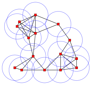
Discrete geometry and combinatorial geometry are branches of geometry that study combinatorial properties and constructive methods of discrete geometric objects. Most questions in discrete geometry involve finite or discrete sets of basic geometric objects, such as points, lines, planes, circles, spheres, polygons, and so forth. The subject focuses on the combinatorial properties of these objects, such as how they intersect one another, or how they may be arranged to cover a larger object.

<span class="mw-page-title-main">Fano plane</span> Geometry with 7 points and 7 lines

In finite geometry, the Fano plane is a finite projective plane with the smallest possible number of points and lines: 7 points and 7 lines, with 3 points on every line and 3 lines through every point. These points and lines cannot exist with this pattern of incidences in Euclidean geometry, but they can be given coordinates using the finite field with two elements. The standard notation for this plane, as a member of a family of projective spaces, is PG(2, 2). Here PG stands for "projective geometry", the first parameter is the geometric dimension and the second parameter is the order.

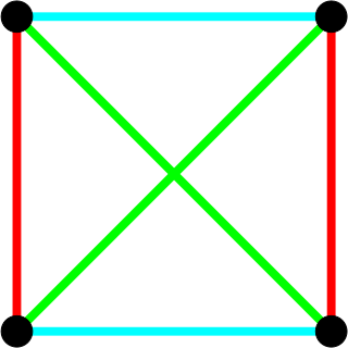
In mathematics, an incidence matrix is a logical matrix that shows the relationship between two classes of objects, usually called an incidence relation. If the first class is X and the second is Y, the matrix has one row for each element of X and one column for each element of Y. The entry in row x and column y is 1 if x and y are related and 0 if they are not. There are variations; see below.

In geometry, a striking feature of projective planes is the symmetry of the roles played by points and lines in the definitions and theorems, and (plane) duality is the formalization of this concept. There are two approaches to the subject of duality, one through language and the other a more functional approach through special mappings. These are completely equivalent and either treatment has as its starting point the axiomatic version of the geometries under consideration. In the functional approach there is a map between related geometries that is called a duality. Such a map can be constructed in many ways. The concept of plane duality readily extends to space duality and beyond that to duality in any finite-dimensional projective geometry.

<span class="mw-page-title-main">Sylvester–Gallai theorem</span> Existence of a line through two points

The Sylvester–Gallai theorem in geometry states that every finite set of points in the Euclidean plane has a line that passes through exactly two of the points or a line that passes through all of them. It is named after James Joseph Sylvester, who posed it as a problem in 1893, and Tibor Gallai, who published one of the first proofs of this theorem in 1944.

In combinatorial mathematics, a block design is an incidence structure consisting of a set together with a family of subsets known as blocks, chosen such that frequency of the elements satisfies certain conditions making the collection of blocks exhibit symmetry (balance). Block designs have applications in many areas, including experimental design, finite geometry, physical chemistry, software testing, cryptography, and algebraic geometry.

<span class="mw-page-title-main">Levi graph</span>

In combinatorial mathematics, a Levi graph or incidence graph is a bipartite graph associated with an incidence structure. From a collection of points and lines in an incidence geometry or a projective configuration, we form a graph with one vertex per point, one vertex per line, and an edge for every incidence between a point and a line. They are named for Friedrich Wilhelm Levi, who wrote about them in 1942.

<span class="mw-page-title-main">Pappus's hexagon theorem</span> Geometry theorem

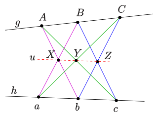
In mathematics, Pappus's hexagon theorem states that

<span class="mw-page-title-main">Incidence geometry</span> Field of mathematics which studies incidence structures

In mathematics, incidence geometry is the study of incidence structures. A geometric structure such as the Euclidean plane is a complicated object that involves concepts such as length, angles, continuity, betweenness, and incidence. An incidence structure is what is obtained when all other concepts are removed and all that remains is the data about which points lie on which lines. Even with this severe limitation, theorems can be proved and interesting facts emerge concerning this structure. Such fundamental results remain valid when additional concepts are added to form a richer geometry. It sometimes happens that authors blur the distinction between a study and the objects of that study, so it is not surprising to find that some authors refer to incidence structures as incidence geometries.

<span class="mw-page-title-main">Configuration (geometry)</span> Points and lines with equal incidences

In mathematics, specifically projective geometry, a configuration in the plane consists of a finite set of points, and a finite arrangement of lines, such that each point is incident to the same number of lines and each line is incident to the same number of points.

<span class="mw-page-title-main">Desargues configuration</span> Geometric configuration of ten points and lines

In geometry, the Desargues configuration is a configuration of ten points and ten lines, with three points per line and three lines per point. It is named after Girard Desargues.

<span class="mw-page-title-main">Möbius–Kantor configuration</span> Geometric structure of 8 points and 8 lines

In geometry, the Möbius–Kantor configuration is a configuration consisting of eight points and eight lines, with three points on each line and three lines through each point. It is not possible to draw points and lines having this pattern of incidences in the Euclidean plane, but it is possible in the complex projective plane.

<span class="mw-page-title-main">Möbius configuration</span>

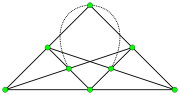
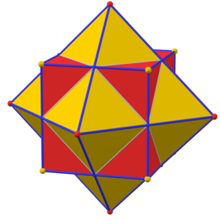
In geometry, the Möbius configuration or Möbius tetrads is a certain configuration in Euclidean space or projective space, consisting of two mutually inscribed tetrahedra: each vertex of one tetrahedron lies on a face plane of the other tetrahedron and vice versa. Thus, for the resulting system of eight points and eight planes, each point lies on four planes, and each plane contains four points.

<span class="mw-page-title-main">Hesse configuration</span> Geometric configuration of 9 points and 12 lines

In geometry, the Hesse configuration is a configuration of 9 points and 12 lines with three points per line and four lines through each point. It can be realized in the complex projective plane as the set of inflection points of an elliptic curve, but it has no realization in the Euclidean plane. It was introduced by Colin Maclaurin and studied by Hesse (1844), and is also known as Young's geometry, named after the later work of John Wesley Young on finite geometry.

In mathematics, the classical Möbius plane is the Euclidean plane supplemented by a single point at infinity. It is also called the inversive plane because it is closed under inversion with respect to any generalized circle, and thus a natural setting for planar inversive geometry.

In geometry, a truncated projective plane (TPP), also known as a dual affine plane, is a special kind of a hypergraph or geometric configuration that is constructed in the following way.

References

  1. Colbourn & Dinitz 2007 , p. 702
  2. 1 2 Dembowski 1968 , pp. 1–2
  3. Biliotti, Jha & Johnson 2001 , p. 508
  4. The term linear space is also used to refer to vector spaces, but this will rarely cause confusion.
  5. Moorhouse 2014 , p. 5
  6. 1 2 Beth, Jungnickel & Lenz 1986 , p. 17
  7. Pisanski & Servatius 2013 , p. 222
  8. E. Steinitz (1894), Über die Construction der Configurationenn3, Dissertation, Breslau
  9. Gropp, Harald (1997), "Configurations and their realizations", Discrete Mathematics, 174: 137–151, doi: 10.1016/s0012-365x(96)00327-5
  10. Levi, F. W. (1942), Finite Geometrical Systems, Calcutta: University of Calcutta, MR   0006834
  11. Coxeter, H.S.M. (1950), "Self-dual configurations and regular graphs", Bulletin of the American Mathematical Society, 56: 413–455, doi: 10.1090/s0002-9904-1950-09407-5
  12. 1 2 Pisanski & Servatius 2013 , p. 158

Bibliography

Further reading